Process Structure in SSAS

By

-

February 12, 2012

Friends,

There are many ways to process a cube but when you are doing Defect Fixing then the best option to test you fix is “Process Structure”. In this post let us discuss about the use of Process Structure processing type.

You can process at different levels like –

Dimensions
Solution
Cube
Partitions

You will find different options at different levels. For example You can find only the following three options while processing at solution level –

Process Full
Process Default
Unprocess

and if you see at dimension level you can see new set(including the set given at solution level) like –

Process Data
Process Index
Process Update

The Hero of the post “Process Structure” is available at Cube level. Before jumping into the topic let’s spend some time on understanding WHAT IS PROCESS ? a worth question to be asked to ourselves.

Processing a cube is very important in SSAS as the end user cannot access the data from Cube database until we process the cube. Cube Processing will do the following things –

Will read data for dimensions and creates indexes
Will read data for Measure Groups
Creates Aggregations

Until the complete Cube processing is done, we cannot access data from cube. While processing, the server READS data for each object(dimension,partitions,mining structures … ) and once the data read is completed it will MARK as PROCESSED for that particular object. When you try to browse data from cube then the server first checks whether the STATE of ALL objects is PROCESSED or not. If not then it will return you a message saying “Cube is not available as it is not completely processed”.

Now let’s come back to our story i.e the advantage of “Process structure”. Let’s say there are 10 dimensions and 3 Measure Groups in you cube and Testing Team raised an issue related to a Measure Group data then the best option to test your FIX is “Process Structure”. “Process Structure” processes all the dimensions and MARK(Yes,Just Marks) all the measure groups as PROCESSED. So, you can browse your cube as all the objects are Marked as Processed. Then you can PROCESS the MEASURE GROUP you want and check the FIX and if everything is fine then you can go ahead in processing the remaining Measure Groups.

Let’s see one more scenario which is from my experience. There were 20 Measure Groups in my last projects and for Processing all the Measure Groups it was taking something around 10 Hours and always ONE Measure Group was creating problem. So the step we followed was –

Process Structure of Cube
Process the Dimension which was creating problem
Validate the Measure Group Data
Process the remaining measure groups

The above method saved lot of time in case of an error as we doesn’t need to process all the partitions to find whether data is coming correct or not. You can find this option under cube Processing options as shown in below Screenshot –

In Simple “Process Structure” is a cheat which marks as Partitions(Measure Groups) as Processed with out actually processing and makes cube available for browsing. This really saves your time while Defect Fixing.

That’s it .. Happy Coding and Please make Full use of “Process Structure” .. 🙂

Regards,

Roopesh Babu V

REFRESH property in SSAS DSV

By

roopesh.valluru

-

February 11, 2012

1156

Friends,

This is very important option provided by Microsoft for SSAS and it is very important interview question too. Don’t expect an interview with out having a question about this REFRESH option. Let’s see complete story about this REFRESH option here.

Firstly, lets see where this option available in SSAS BIDS environment. You can find this in Data Source View in short DSV. IIf you open DSV and right click on Vacant area then you can see context menu items among which one is “Refresh”. PFB screenshot showing the Refresh option in DSV.

Now let’s see the use of this option. Let’s say I added 10 tables to my DSV and dimensions and Measure groups are defined and the cube is built. Now I got a new requirement which lead to structural changes of the tables that are used in DSV. Structural changes includes

1) Adding a column to a table or view

2) Deleting a Column

3) Removing or adding Primary Keys

4) Removing or Adding Relationships

If you wish to get all the structural changes happened to the tables that are part of DSV then REFRESH is the option. If you click on REFRESH then it will check in database for changes happened to the tables in DSV and will prompt us to Add the changes to DSV.

Example – In the DSV shown in the below screenshot a table “DimCustomer” is added.

Now I am adding a new column to this table in Database with the name “Address” using the below query –

Alter table DimGeography
Add Address Varchar(100)

To pull this column into DSV table I can do the following things.

Removing Table from DSV and Adding it back
Using Refresh Option

If you use the First option listed above and when u remove the table from DSV then all the objects created like Dimensions,Measure Groups,Relations .. using this table will get deleted. This will be very risky and not a best option to pull the changes into Cube. So, The best option is using Refresh button. If you select refresh option then it will show you the changes occurred in database level as shown in below screenshot –

If you select OK then the changes will be updated to the tables in DSV. The only Disadvantage with this option is you have to accept all the changes or reject all the changes. You cannot accept partial changes by rejecting the remaining. Either Full or Null.

That’s it .. Happy Coding !!

Regards,

Roopesh Babu V

Axis in MDX

By

roopesh.valluru

-

February 11, 2012

421

Friends,

Most important function of MDX is AXIS. The Axis function returns a set of tuples on the specified axis. PFB syntax of AXIS function.

“Axis(Number)”

Number – is a valid numeric expression which specifies the axis number.

The position starts from 0 and it can be continued as the cube database data is MULTI dimensional. MDX query is capable of returning data in more than two dimensions but our systems doesn’t support it. As our systems support only up to two dimensions, our MDX queries will stick to two AXIS only. For example, Axis(0) returns the COLUMNS axis, Axis(1) returns the ROWS axis, and so on. The Axis function cannot be used on the filter axis. The Axis numbers should be in order. You cannot use AXIS(1) without defining AXIS(0). PFB the sequence –

AXIS(0) or simply 0 – Columns

AXIS(1) or simply 1 – Rows

AXIS(2) or simply 2 – Pages

AXIS(3) or simply 3 – Sections

……….

You can use any format to define AXIS like AXIS(Number) or Simply Number or with name like columns,rows,pages .. PFB sample queries of all three kinds –

Using AXIS –

select [Measures].[Sales Amount] on Axis(0),
[Dim Product].[Products].[Products] on Axis(1)
From [Adventure Works]

Using Number –

select [Measures].[Sales Amount] on 0,
[Dim Product].[Products].[Products] on 1
From [Adventure Works]

Using Name –

select [Measures].[Sales Amount] on Columns,
[Dim Product].[Products].[Products] on Rows
From [Adventure Works]

For all the above three queries the result set is same and the screenshot of the same is shown below –

That’s the complete story about AXIS function and hope you understood the concept. Happy Coding !!

Regards,

Roopesh Babu V

BottomCount in MDX

By

roopesh.valluru

-

February 11, 2012

147

Friends,

This function is very much similarly to the functions BottomSum and BottomPercent. Please find the Major Difference between the all three functions –

1) BottomCount – Orders the set and then returns specified number of tuples in the specified set with the lowest values will be pulled.

2) BottomPercent – Orders the set and then returns tuples from the bottom of the set with the lowest values whose cumulative total is less than or equal to the supplied percentage.

3) BottomSum – Orders the set and then returns the summed value of a numeric expression across a supplied set.

In this post we are gonna discuss about BottomCount Function. This function will do TWO jobs

1) Sorts the set based on numeric parameter in Ascending order.

2) Returns specified number of tuples in the specified set with the lowest values.

PFB the syntax of the same.

BottomCount(Set_Exp,Count,Numeric_Exp).

Set_Exp – Valid MDX Set Expression

Count – It specifies the NUMBER of records to be returned.

Numeric_Exp – NOT A MANDATORY PARAMETER and it specifies on what column basis the set needs to be ordered.

If the numeric expression is specified then BottomCount is nothing by the combination of TWO MDX functions i.e ORDER(Asc) + TAIL and if the numeric expression is not specified then it is JUST like TAIL function in MDX.

If the numeric expression is specified then the set specified in the function will get sorted according to the value of the specified numeric expression in ascending order and then returns the specified number of tuples from BOTTOM.

Now lets see the difference between two cases –

In the below case I specified Numeric Expression and the below query returns 10 “Products” that have the lowest “Sales Amount”.

select [Measures].[Sales Amount] on Columns,
BottomCount([Dim Product].[Products].[Products],10,[Measures].[Sales Amount]) on Rows
From [Adventure Works]

If you see the screenshot given below, it is returning all NULLS as in most of the cases you will have products with NO SALES and as we are requesting for BottomCount it will return Products with LEAST values and obviously NULLS.

The above one is correct but none of the client wants to see the least valued products which has NO SALES at all instead they wish to see least valued products whose sales is NON ZERO. PFB the query which will return the bottom products with NON ZERO sales.

select [Measures].[Sales Amount] on Columns,
BottomCount(FILTER([Dim Product].[Products].[Products], NOT ISEMPTY([Measures].[Sales Amount])),
10,[Measures].[Sales Amount]) on Rows
From [Adventure Works]

In the above query I am filtering EMPTY records and pfb the screenshot of the output.

The above output looks perfect and for sure client will be happy. he will be even more happy if you format the output .. 😉 Now let’s see the other scenario i.e with out giving numeric expression and pfb sample query of the same –

select [Measures].[Sales Amount] on Columns,
BottomCount([Dim Product].[Products].[Products],10) on Rows
From [Adventure Works]

In the above query no Numeric expression to ask server to SORT the set in an order before returning 10 records. The output is as shown in below screenshot –

The above output is entirely different from the previous one as the last one is not sorting the data before selecting the records. If the see the products names you can see that the products are ordered alphabetically and then returning last 10.

So, in simple BottomCount with numeric_Exp is Order(ASC) + Tail and BottomCount without numeric_Exp acts like TAIL function.

That’s it .. Happy Coding !!

Regards,

Roopesh Babu V

How to Repeat a Table in every page of SSRS Report

By

roopesh.valluru

-

February 8, 2012

446

Friends,

Lets say we have to show summarized data and detailed data in a report and the summarized data should repeat on all the pages of the report. This is quite common requirement that clients are asking for. Let’s see how to acheive this. There are many ways of doing this but I will demonstrate one way here i.e making use of property “Repeat Page Header”. I have choosen Adventure Works database which is available in almost all computers who are working or learning MSBI. PFB the steps that you have to follow to acheive the same.

Take a Report and add Data Source.
Define a dataset and pfb the Screenshot of the query I am using to demonstrate the same here.

Take two TABLE controls into the report and add the data fields as shown below.

For the first table I added a ROW GROUP to show summarized data and here we are grouping data based on English Product Category Name as shown in below pic.

If you Preview the report then it will have two tables one with summarized data and other with detailed data as shown below.

In the above screen shot we can clearly see the summarized table and detailed table and clients want to see this summarized table in all the pages. Now Merge all the cells of the header of TABLE 2 by selecting all HEADER columns and by selecting the menu item MERGE which is present on RIGHT CLICK as shown in the below screenshot.

Delete the Header text of Table 2 and CUT the table 1 and PASTE it on Merged Header part and align the columns as shown in below screenshot.

Now Select the Table 2 and set the property “RepeatColumnHeaders” to TRUE.
Now click on the SMALL TRIANGLE on Groups and click on “Advanced Mode” and once you select that you can see STATIC in Row Groups and Column Groups as shown below.

Select STATIC item from Row Groups section and press F4 for properties and select “RepeatonNewPage” to TRUE as shown below.

Now Preview the report and you can see t able on data in all the pages as shown in below Screenshot.

In the above screenshot we can clearly see that the TABLE 1data is repeating for all the pages. This is one way of repeating table data in all the pages of the report. Look and Feel is in your hands and you can design as per your requirements.

That’s it .. Happy Coding !!

Regards,

Roopesh Babu V

Ascendants Function in MDX

By

roopesh.valluru

-

February 6, 2012

256

Friends,

Lets discuss about Ascendants Function here. This function is very close to Ancestor and Ancestors functions but the major differences are both Ancestor and Ancestors returns the items at the specified level where as Ascendants returns items from all the levels including the member itself. PFB the syntax of the same –

Ascendants(Member_Expression)

You can see from the above syntax that there is no SECOND parameter like in Ancestor/Ancestors as it returns Ancestors of all the levels. Lets say we have a TIME Hierarchy as shown below.

Year –> Semester –> Quarter –> Month.

If you use Ascendants function to a member at Month level then the output will contain –

Month Member -> Month’s Parent(Quarter) -> Quarter’s Parent(Semester) -> Semester’s Parent(Year)

This is why we doesn’t need SECOND parameter to specify LEVEL like in Ancestor/Ancestors function. Ascendants returns the set of the ascendants of a specified member, including the member itself. So,The Ascendants function returns all of the ancestors of a member from the member itself up to the top of the member’s hierarchy; more specifically, it performs a post-order traversal of the hierarchy for the specified member, and then returns all ascendant members related to the member, including itself, in a set. This is in contrast to the Ancestor function, which returns a specific ascendant member, or ancestor, at a specific level.

PFB sample query using Ascendants Function –

select [Measures].[Sales Amount] on Columns,
Ascendants([Dim Time].[Hierarchy].[Calendar Year].&[2002].&[3].&[September]) on Rows
From [Adventure Works]

In the above query I am asking for Ascendants of “[Dim Time].[Hierarchy].[Calendar Year].&[2002].&[3].&[September]” member which belongs to MONTH level of Hierarchy and the result set looks like in the below given screenshot –

Tip – So, When you want Ancestors at a Specified level then go with Ancestor where as if your requirement is to pull complete Family of a Member then use Ascendants function.

That’s it .. Happy Coding !!

Regards,

Roopesh Babu V

Ancestors Function in MDX

By

roopesh.valluru

-

February 6, 2012

4

Friends,

This is Very similar to the Function Ancestor in MDX. The major difference is that Ancestor returns Ancestor where as Ancestors returns SET OF ALL ANCESTORS at the specified level. With Microsoft SQL Server Analysis Services, the set returned will always consist of a single member – Analysis Services does not support multiple parents for a single member. So, this is not a useful one in SSAS MDX. This function works on Hierarchies. If you pass a member and a level then it will return the ALL the ANCESTORS of a specified member at a specified level. PFB the syntax of the Ancestors function.

Ancestors(Member_Expression,Level_Expression)

Member_Expression – A valid MDX expression that returns a member from a Hierarchy Level.

Level_Expression – A valid MDX expression that returns a level from a Hierarchy Level.

For Ancestors function when you pass a member from a level of hierarchy then the level parameter value can be any from the same hierarchy but it should be above the level to which the member belongs. For example consider time hierarchy –

Year –> Quarter –> Month

If you pass a member from Quarter level then the level parameter should be either Quarter and Year but not Month. If a level expression is specified, the Ancestors function returns ALL the MEMBERS(PARENTS) of specified member at the specified level. If the specified member is not within the same hierarchy as specified level, the function returns an error.

You can also specify Distance instead of LEVEL as parameter. If a distance is specified, the Ancestors function returns ALL the ANCESTORS of the specified member that is the number of steps specified up in the hierarchy specified by the member expression. A member may be specified as a member of an attribute hierarchy, a user-defined hierarchy, or in some cases, a parent-child hierarchy. A number of 1 returns a member’s parent and a number of 2 returns a member’s grandparent (if one exists). A number of 0 returns the member itself. The syntax looks like given below –

Ancestors(Member_Expression,Distance)

PFB the query sample which is using Level_Expression –

select [Measures].[Sales Amount] on Columns,
Ancestors([Dim Time].[Hierarchy].[Calendar Year].&[2002].&[3].&[September],[Dim Time].[Hierarchy].[Calendar Quarter]) on Rows
From [Adventure Works]

PFB the same query as above but using Distance –

select [Measures].[Sales Amount] on Columns,
Ancestors([Dim Time].[Hierarchy].[Calendar Year].&[2002].&[3].&[September],1) on Rows
From [Adventure Works]

In the above Screenshot you can clearly see that Ancestors function is also returning a SINGLE value as Many parents are not allowed in SSAS. You can use Ancestors function to navigate to any level above to the level to which the member passed as parameter belongs to. There is one more function which acts in the same fashion i.e Parent. Learn more about Parent Function here.

That’s it .. Happy Coding !!

Regards,

Roopesh Babu V

Ancestor Function in MDX

By

roopesh.valluru

-

February 6, 2012

84

Friends,

In this post we are gonna discuss about a Navigation function i.e Ancestor. This function works on Hierarchies. If you pass a member and a level then it will return the ancestor of a specified member at a specified level. PFB the syntax of the Ancestor function.

Ancestor(Member_Expression,Level_Expression)

Member_Expression – A valid MDX expression that returns a member from a Hierarchy Level.

Level_Expression – A valid MDX expression that returns a level from a Hierarchy Level.

For Ancestor function when you pass a member from a level of hierarchy then the level parameter value can be any from the same hierarchy but it should be above the level to which the member belongs. For example consider time hierarchy –

Year –> Quarter –> Month

If you pass a member from Quarter level then the level parameter should be either Quarter and Year but not Month. If a level expression is specified, the Ancestor function returns the ancestor of specified member at the specified level. If the specified member is not within the same hierarchy as specified level, the function returns an error.

You can also specify Distance instead of LEVEL as parameter. If a distance is specified, the Ancestor function returns the ancestor of the specified member that is the number of steps specified up in the hierarchy specified by the member expression. A member may be specified as a member of an attribute hierarchy, a user-defined hierarchy, or in some cases, a parent-child hierarchy. A number of 1 returns a member’s parent and a number of 2 returns a member’s grandparent (if one exists). A number of 0 returns the member itself. The syntax looks like given below –

Ancestor(Member_Expression,Distance)

PFB the query sample which is using Level_Expression –

select [Measures].[Sales Amount] on Columns,
Ancestor([Dim Time].[Hierarchy].[Calendar Year].&[2002].&[3].&[September],[Dim Time].[Hierarchy].[Calendar Quarter]) on Rows
From [Adventure Works]

PFB the same query as above but using Distance –

select [Measures].[Sales Amount] on Columns,
Ancestor([Dim Time].[Hierarchy].[Calendar Year].&[2002].&[3].&[September],1) on Rows
From [Adventure Works]

You can use Ancestor function to navigate to any level above to the level to which the member passed as parameter belongs to. There is one more function which acts in the same fashion i.e Parent. Learn more about Parent Function here.

That’s it .. Happy Coding !!

Regards,

Roopesh Babu V

AllMembers Function in MDX

By

roopesh.valluru

-

February 6, 2012

1066

Friends,

This will be used at either Hierarchy or Level of an attribute. Let us First see what is this Hierarchy and Levels. Lets say I have a dimension named “Time” and attributes Year,Quarter and Month. Then each attribute will be represented as shown below.

[Time].[Year].[Year]
[Time].[Quarter].[Quarter]
[Time].[Month].[Month]

Each representation has three parts and the generalized representation of an attribute is <Dimension>.<Hierarchy>.<Level>. So the levels will be splitted as ollows.

<Dimension> – Dimension level
<Dimension>.<Hierarchy> – Hierarchy Level
<Dimension>.<Hierarchy>.<Level> – Level Level

Now lets come back to AllMembers Function and this mainly used at Hierarchy and Level levels. Lets see the syntax of both.

<Hierarchy_Exp>.AllMembers

<Level_Exp>.AllMembers

The AllMembers function returns a set that contains all members, which includes calculated members, in the specified hierarchy or level. The AllMembers function returns the calculated members even if the specified hierarchy or level contains no visible members.

PFB the sample query at Hierarchy level –

SELECT {} ON COLUMNS,
{[Time].[Year].AllMembers} ON ROWS
FROM [Adventure Works]

The above query returns all the members of the Year hierarchy. It is given at Hierarchy level and hence ALL member will also be returned if the “IsAggregatable” Property of this attribute is set to TRUE in BIDS.

PFB the sample query at Level level –

SELECT {} ON COLUMNS,
{[Time].[Year].[Year].AllMembers} ON ROWS
FROM [Adventure Works]

The above query returns all the members of the Year level. It is given at Hierarchy level and hence ALL member will NOT be returned.

When a dimension contains only a single visible hierarchy, the hierarchy can be either referred to by the dimension name or by the hierarchy name, because the dimension name in this case is resolved to its only visible hierarchy. For example, Measures.AllMembers is a valid MDX expression because it resolves to the only hierarchy in the Measures dimension and this AllMembers function is semantically similar to the AddCalculatedMembers (MDX) function when you use on MEASURES HIERARCHY. PFB sample query for the same.

select Measures.AllMembers on Columns,
[Dim Time].[Calendar Year].&[2004] on Rows
From [Adventure Works]

PFB the screenshot of the same –

That’s it .. Hope you understood the concept .. Happy Coding !!

Regards,

Roopesh Babu V

AddCalculatedMembers in MDX

By

roopesh.valluru

-

February 5, 2012

1

Friends,

AddCalculatedMembers function helps you in retrieving all the calculated members data in the result set. We have to pass a Set_Expression as parameter to this function and this returns a set generated by adding ALL the calculated measures to the set specified in Function. PFB the syntax of the same –

AddCalculatedMembers(Set_Expression)

Lets see a simple query which returns complete measures data in the result set.

select {Measures.members} on Columns,
[Dim Time].[Calendar Year].&[2004] on Rows
from [Adventure Works]

In the above query we specified {Measures.members} on Columns and hence it returns all the measures EXCEPT Calculated Measures. To confirm the same please check the below screenshot in which it is clear that all the measures are pulled as part of result set EXCEPT Calculated Measures.

Now lets use the same query by adding AddCalculatedMembers Function to it. PFB the updated query –

select AddCalculatedMembers(Measures.members) on 0,
[Dim Time].[Calendar Year].&[2004] on 1
from [Adventure Works]

Now the calculated member which was not part of last output will also be retrieved as shown below.

By default, MDX excludes calculated members when it resolves set functions. The AddCalculatedMembers function examines the set expression specified in Set_Expression,and includes calculated members that are siblings of the members contained within the scope of that set expression.

Note that it is not mandatory that you have to use retreive all MEASURES in order to pull calculates members. In simple itis not mandatory to use Measures.Members as parameter of the function. You can simply use any valid SET expression and in the below query I am demonstrating the same with ONE Measure.

select AddCalculatedMembers([Measures].[Sales Amount]) on 0,
[Dim Time].[Calendar Year].&[2004] on 1
from [Adventure Works]

The above query pulls ALL the calculated members along with “Sales Amount” measure as shown below.

Tip – There is a way to PULL ONLY calculated members excluding all the measures and PFB the query sample for the same.

select AddCalculatedMembers(Measures.Members) – Measures.Members on 0,
[Dim Time].[Calendar Year].&[2004] on 1
from [Adventure Works]

In the above query in the first set we are pulling all the measures and calculated members and we are excluding the measures from the resultant set. The below query also helps you in acheiving the same but for the below query You need to know atleast one measure name in the cube.

select AddCalculatedMembers([Measures].[Sales Amount]) – [Measures].[Sales Amount] on 0,
[Dim Time].[Calendar Year].&[2004] on 1
from [Adventure Works]

I am pulling all the calculated members + Sales Amount and then removing Sales Amount measure from the result set.

Alert – Instead of this function you can use another function to retrieve the same result as AddCalculatedMembers function i.e AllMembers. PFB the query for the same.

select Measures.AllMembers on 0,
[Dim Time].[Calendar Year].&[2004] on 1
from [Adventure Works]

That’s it and hope you understood the concept and Happy Coding !!

Regards,

Roopesh Babu V

LAG Function in MDX

By

roopesh.valluru

-

February 5, 2012

637

Friends,

If you have read the article about LEAD then you wil easily say that LAG is just opposite to LEAD function after finished reading this article. LAG is a Navigation Function which returns a value(member) that is N number of positions following the supplied member in the given attribute. Typical uses of this function is to navigate back or forward to N positions from the given member. PFB the syntax of LEAD function –

Member_Expression.Lag(Index)

Member_Expression - A valid Attribute Member .

Index - The number of positions we wish to navigate.

Member positions within a level are determined by the attribute hierarchy’s natural order. The numbering of the positions is zero-based. If the specified lead is zero (0), the Lead function returns the specified member. If you specified 1(One) then it will take you backward by one Member, if 2(Two) then will navigate backward by two members from the current member.

Positive Lag and Negative Lag –

If you specify a POSITIVE number as Index then it will go backward from the current member and this is called POSITIVE LAG. Lets see an example for Positive Lag here.

Select [Date].[Fiscal].[Month].[January 2001].Lag(5) on 0

from [Adventure Works].

If you see the above query member expression is “[Date].[Fiscal].[Month].[January 2001]” and current member is “January 2001”. We have given Lag(5) and hence it will navigate back by FIVE members and will return “August 2000” as output if that member exists in Cube.

If you specify a NEGATIVE number as Index then it will go forward from the current member and this is called NEGATIVE LAG. Lets see an example for Negative Lag here.

Select [Date].[Fiscal].[Month].[January 2001].LAG(-5) on 0

from [Adventure Works].

If you see the above query member expression is “[Date].[Fiscal].[Month].[January 2001]” and current member is “January 2001”. We have given Lag(-5) and hence it will navigate forward by FIVE members and will return “June 2001” as output if that member exists in Cube.

PFB screenshot which shows an example for Lag function.

Note – Lag looks like a simple function and not much useful one in real time scenarios but this function in combination with other functions like CLOSING PERIOD or RANGE functions will be most powerful and useful one.

Remember – Positive Lead = Negative Lag and Negative Lead = Positive Lag

That’s it .. Happy Coding !!

Regards,

Roopesh Babu V

LEAD Function in MDX

By

roopesh.valluru

-

February 5, 2012

643

Friends,

If you have read the article about LAG then you will easily say that LEAD is just opposite to LAG function after finished reading this article.LEAD is a Navigation Function which returns a value(member) that is N number of positions following the supplied member in the given attribute. Typical uses of this function is to navigate back or forward to N positions from the given member. PFB the syntax of LEAD function –

Member_Expression.Lead(Index)

Member_Expression - A valid Attribute Member .

Index - The number of positions we wish to navigate.

Member positions within a level are determined by the attribute hierarchy’s natural order. The numbering of the positions is zero-based. If the specified lead is zero (0), the Lead function returns the specified member. If you specified 1(One) then it will take you forward by one Member, if 2(Two) then will navigate forward by two members from the current member.

Positive Lead and Negative Lead –

If you specify a POSITIVE number as Index then it will go forward from the current member and this is called POSITIVE LEAD. Lets see an example for Positive Lead here.

Select [Date].[Fiscal].[Month].[January 2001].Lead(5) on 0

from [Adventure Works].

If you see the above query member expression is “[Date].[Fiscal].[Month].[January 2001]” and current member is “January 2001”. We have given LEAD(5) and hence it will navigate forward by FIVE members and will return “June 2001” as output if that member exists in Cube.

If you specify a NEGATIVE number as Index then it will go back from the current member and this is called NEGATIVE LEAD. Lets see an example for Negative Lead here.

Select [Date].[Fiscal].[Month].[January 2001].LEAD(-5) on 0

from [Adventure Works].

If you see the above query member expression is “[Date].[Fiscal].[Month].[January 2001]” and current member is “January 2001”. We have given LEAD(-5) and hence it will navigate back by FIVE members and will return “August 2000” as output if that member exists in Cube.

PFB screenshot which shows an example for Lead function.

Note – Lead looks like a simple function and not much useful one in real time scenarios but this function in combination with other functions like CLOSING PERIOD or RANGE functions will be most powerful and useful one.

Remember – Positive Lead = Negative Lag and Negative Lead = Positive Lag.

That’s it .. Happy Coding !!

Regards,

Roopesh Babu V

Named Query in SSAS DSV

By

roopesh.valluru

-

February 5, 2012

333

Friends,

Here we are gonna discuss about Named Queries. This is one of the important property in SSAS DSV. A Named Query is nothing but a simple VALID SQL expression. In a named query, you can specify an SQL expression to select rows and columns returned from one or more tables in one or more data sources. A named query is like any other table in a data source view with rows and relationships, except that the named query is based on an expression. The main advantage of this Named Query is that it gives you power to change the structure of tables and views that are present in data source but with out modifying the same in data source i.e the changes you are making to any object of the Database will be at DSV level only. The underlying objects in database will remain in the same condition.

Lets see a simple example. Let’s say there are three tables table1,table2 and table3 then you can use a SQL statement which joins all the three tables and pulls only required columns and create a Named Query with it. The output of this one will become a brand new table with required columns. Lets see the steps involved in creating a named query.

1) Create a DS.

2) Create an empty DSV.

3) Right click on DSV and select New Named Query option as shown below.

4) Give some meaningful name and Add tables required or directly copy and past the query in the bottom last pane then click on OK.

That’s it. A new named query is created. Remember that You can use complex queries as well as simple queries but it should be a valid SQL expression. PFB the example for a simple Expression.

Select Getdate().

Yup, the above expression is valid to create a named query and it returns Server System current date. Hope you understood the concepts and Happy Coding Guys !!

Regards,

Roopesh Babu V

Impersonation in SSAS Data Source

By

roopesh.valluru

-

February 5, 2012

326

Friends,

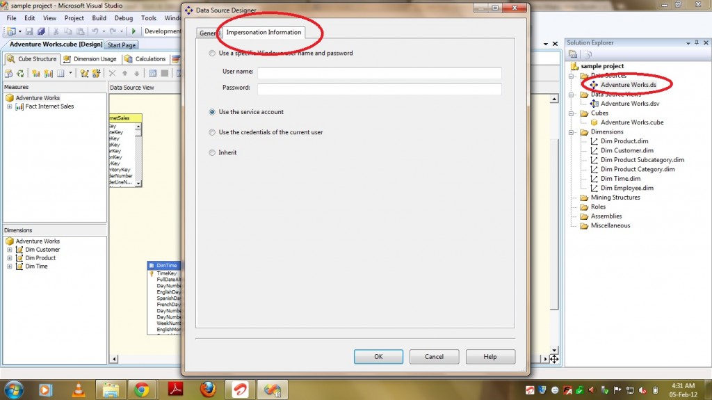
We are gonna discuss about the use of Impersonation tab in Data Source wizard of SSAS solution in this post. First lets discuss about WHY we need to impersonate and then different types in which we can impersonate.

When we design a cube in which data source is using windows authentication then it will be executed as current user. But, when you deploy the database to the server there will be no current user. In this case when a user requests AS to process an object it needs to know under what security context to connect to the data source. Essentially you need to get the AS service to impersonate another user in order to retrieve data from an external source on a user’s behalf.

There are FOUR types available in which you can impersonate Data Source.

1) Use a specific Username and Password.

2) Use the Service Account.

3) Use the credentials of the Current User.

4) Inherit (in SQL 2008 and above)/ Default (SQL 2005).

Now lets see where you can provide this impersonation information in SSAS Solution.

1) Open New Solution.

2) Add New Data Source.

3) Provide Database connectivity Details.

4) After providing data source details if you click on next then you can see a Wizard page to provide impersonate info for the data source as shown below.

Now lets see in detail the use of each impersonation type.

Use a specific Username and Password –

Select this option to have the Analysis Services object use the security credentials of a specified Windows user account.

• User name – Type the domain and name of the user account to be used by the selected Analysis Services object. The domain and name of the user account uses the following format:
<Domain name>\<User account name>
• Password – Type the domain and name of the user account to be used by the selected Analysis Services object.

When Analysis Services account does not have relational data base access then Use Specific User Name and password option is used.
Specific user name and password is passed to analysis server but it will be encrypted due to security. Example like when the data sources are like –
1) OLE DB/Microsoft Directory Services
2) SQL Server Compact Edition

Use the Service Account –

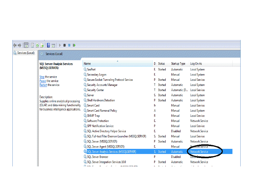
Select this option to have the Analysis Services object use the security credentials associated with the Analysis Services service that manages the object. The service account credentials will be used for processing, ROLAP queries, remote partitions, linked objects, and synchronization from target to source. For DMX OPENQUERY statements, local cubes, and mining models, the credentials of the current user will be used. This option is not supported for out-of-line bindings.

“Use the Service Account” option is mostly used by developers. In this, Analysis Services startup account information will be used to connect relational database.

Use the credentials of the Current User –

This is similar to the first option what we discussed i.e Specify a user account. If you selects this option then it will take the current logged in user details. Remember that this option is not supported for processing, ROLAP queries, remote partitions, linked objects, and synchronization from target to source.

Default/Inherit –

Analysis services will have Service Account and User Account. If you select this option then it will take the details of default user account . This option uses the default setting for the database for processing objects, synchronizing servers, and executing the OpenQuery data mining statements.

So guys, based on requirement Pick the best one that suits you. Happy Coding !!

Regards,

Roopesh Babu V

Star Schema and Snow Flake Schema

By

roopesh.valluru

-

February 1, 2012

364

Friends,

I have never taken and also given an interview on SSAS(even on MSBI) with out the question “What is the difference between STAR and SNOWFLAKE Schema”. Before going to the differences lets have a look at what a schema is and the types.

Schema in relational database defines the tables, columns in each table, and the relationships between tables. It gives a clear picture about the tables present in the database how the tables are related to each other. There are mainly two types of schema(and ppl are adding one per day like STARFLAKE,GALAXY and so on .. but not to worry much about those) which are listed below.

1) Star

2) SnowFlake.

Lets discuss about each type in detail here.

Star –

This is the simplest Schema design available and in the star schema design, a single object (the fact table) sits in the middle and is radially connected to other surrounding objects (dimension lookup tables) like a star. Each dimension is represented as a single table. The primary key in each dimension table is related to a foreign key in the fact table. In simple when ALL the DIMENSION TABLES are DIRECTLY related to FACT TABLE then that Schema is called as Star Schema. PFB the Screenshot showing STAR Schema.

Snow Flake –

The snowflake schema is an extension of the star schema, where each point of the star explodes into more points. In a star schema, each dimension is represented by a single dimensional table, whereas in a snowflake schema, that dimensional table is normalized into multiple lookup tables, each representing a level in the dimensional hierarchy. When ALL the dimension tables are NOT directly related to FACT table then that type of schema is called as Snow Flake Schema. PFB Screenshot of Snow Flake Schema.

In snow flake schema fact table will be linked directly as well as there will be some intermediate dimension tables or Fact less Fact tables between fact and dimension tables.

That’s it .. Happy Coding !!

Regards,

Roopesh Babu V

No mapping between account names and security IDs was done

By

roopesh.valluru

-

February 1, 2012

271

Friends,

“No mapping between account names and security IDs was done” – This error occurs very rarely. When you defined a ROLE and if you add members to that ROLE then only the chance of occurring this error is there. When you created a role and added Members and Groups to that role and if any of the user is not available in the environment where we are trying to deploy the cube then this error will be thrown by SSAS Server. If you see the below given image, in that I added an user named Lenovo to the role created. Then I removed that user from my machine.

After removing the user added to the role when I try to process(or simply deploy) the cube then it throws the error “No mapping between account names and security IDs was done“. The solution for solving this error is to remove the members and groups who are not available in the environment where we are deploying.

Suggestion – Better to DEFINE role and add members once the cube is completely processed and moved to Production.

That’s it .. Happy Coding !!

Regards,

Roopesh Babu V

What is HOLAP and its advantages and Disadvantages?

By

roopesh.valluru

-

January 31, 2012

36

Hybrid Online Analytical Processing (HOLAP) – HOLAP is a combination of MOLAP and ROLAP. HOLAP stores the detail data in the relational database but stores the aggregations in multidimensional format. Because of this, the aggregations will need to be processed when changes are occur. With HOLAP you will have medium query performance: not as slow as ROLAP, but not as fast as MOLAP. If, however, you were only querying aggregated data or using a cached query, query performance would be similar to MOLAP. But when you need to get that detail data, performance is closer to ROLAP.

Advantages:

HOLAP is best used when large amounts of aggregations are queried often with little detail data, offering high performance and lower storage requirements.
Cubes are smaller than MOLAP since the detail data is kept in the relational database.
Processing time is less than MOLAP since only aggregations are stored in multidimensional format.
Low latency since processing takes place when changes occur and detail data is kept in the relational database.

Disadvantages:

As slow as ROLAP when you try to access leaf level data.
Need to process when new records inserted.

What is ROLAP and its advantages and Disadvantages?

By

roopesh.valluru

-

January 31, 2012

343

ROLAP (Relational Online Analytical Processing) – ROLAP does not have the high latency disadvantage of MOLAP. With ROLAP, the data and aggregations are stored in relational format. This means that there will be zero latency between the relational source database and the cube. When we talk about ROLAP we have to discuss about disadvantage it has. Just because of this disadvantage the usage of ROLAP storage is some thing around 5%.

Disadvantages:

Main Disadvantage of this mode is the performance, this type gives the poorest query performance because no objects benefit from multidimensional storage.

Advantages:

Since the data is kept in the relational database instead of on the OLAP server, you can view the data in almost real time.
Also, since the data is kept in the relational database, it allows for much larger amounts of data, which can mean better scalability.
Low latency.

What is MOLAP and its advantages and disadvantages?

By

roopesh.valluru

-

January 31, 2012

1634

MOLAP stands for Multi dimensional Online Analytical Processing. MOLAP is the most used storage type. It is designed to offer maximum query performance to the users. The data and aggregations are stored in a multidimensional format, compressed and optimized for performance. When a cube with MOLAP storage is processed, the data is pulled from the relational database, the aggregations are performed, and the data is stored in the AS database in the form of binary files. The data inside the cube will refresh only when the cube is processed, so latency is high.

Advantages:

Since the data is stored on the OLAP server in optimized format, queries (even complex calculations) are faster than ROLAP.
The data is compressed so it takes up less space.
And because the data is stored on the OLAP server, you don’t need to keep the connection to the relational database.
Cube browsing is fastest using MOLAP.

Disadvantages:

This doesn’t support REAL TIME i.e newly inserted data will not be available for analysis untill the cube is processed.

What are the different types of storage modes?

By

roopesh.valluru

-

January 31, 2012

8

There are three standard storage modes in OLAP applications.

1) MOLAP

2) ROLAP

3) HOLAP

When ever the cube process is going on then it process leaf level data(detailed data) and creates Aggregations based on the Aggregation design defined in the cube. Now lets see about these in detail –

MOLAP – Stores Detailed data and Aggregations in the form of binary files and these are completely separate from relational database.

ROLAP – Stores Detailed data and Aggregations in the relational database.

HOLAP – Stores Detailed data in relational database and Aggregations in the form of binary files.

PFB the difference between these three –

Storage Mode	Storage Location for Detail Data	Storage Location for Summary/ Aggregations	Storage space requirement	Query Response Time	Processing Time	Latency
MOLAP	Multidimensional Format	Multidimensional Format	MediumBecause detail data is stored in compressed format.	Fast	Fast	High
HOLAP	Relational Database	Multidimensional Format	Small	Fast for aggregated data and Slow when trying to read Leaf level data.	Fast	Medium
ROLAP	Relational Database	Relational Database	Large	Slow	Slow	Low

There is one main difference between ROLAP and MOLAP i.e ROLAP supports REAL TIME Data where as MOLAP doesn’t. Real time in the sense when a record is inserted into fact table then it should be immediately available for analysis. It doesnot happen if you use MOLAP storage mode and to pull newly added record in MOLAP storage mode we need to process cube. In ROLAP as the data is storing in relational databases, when ever a record is inserted into table it will be available for analysis.

Regards,

Roopesh Babu V