Home Blog Page 9

Row Sampling Transformation in SSIS with Example

392

Friends,

This is very much similar to Percentage Sampling with only difference that Row sampling will Limit records by the integer value we passed where as Percentage Sampling takes the %ge of records.

If 1000 records in my source then

Row Sampling – If I take 10 as value then output is 10 records

Percentage Sampling – If I take 10 as value then 10% of 1000 i.e 100 records will be the output.

Lets see an example. You wil feel like you are going through the same Percentage Sampling again if you already read Percentage Sampling.

  • Open a new project and drag a Data Flow task from toolbox in Control Flow.
  • Edit the Data Flow task by double clicking the object or by selecting EDIT button on Right click on the object.
  • Make sure the Data Flow Page is opened as shown below.

  • Select OLE DB data source from data flow sources and drag and drop it in the data flow.
  • Double click on the OLE DB data source to open a new window where we can set the properties of the connection.
  • Select the connection manager and click on new button to set the connection string as shown below.

  • Set the connection to the database by providing the Server name,database name and authentication details if required.
  • After the connection is set, select Data Access mode as “Table or View” as shown below and then select the table which we are gonna use as input to PERCENTAGE SAMPLING Transformation.

  • Now select the columns that needs to be present as part of source by going to Columns Page in OLE DB Data Source as shown below.

  • Now drag and drop Row Sampling transformation and connect OLE DB source output as input to this transformation as shown below.

  • Now edit the Rowsampling transformation and select Number of rows out of total records in the Source table you wants to use as sample by mentioning  it “Number of rows”.
  • Give some meaningful names to Sample Output and Unselected output and use “Use the following random seed” option to get Random values from the source rather than getting TOP records.

  • These are all the properties we can set for Row Sampling transformation. Now lets create couple of destinations to store Sampled output and not sampled output. I have taken OLE DB destination to push Sampled output and Flat File destination to push non sampled output.
  • Now drag the output of Row Sampling transformation to give source to OLE DB destination and it will prompt us to select the INPUT (we have two, one sampled and another one not sampled) and select Sampled output.
  • Select the Non Sampled output to Flat file destination and set the connection settings for both OLE DB and Flat File destinations. (You can see configuring destinations in the post here)
  • Now the package is ready to execute and do the same. Make sure all the items turn GREEN.

  • You can observe the records from source got grouped into two different pipelines based on the Integer we have given.

This is it !! This is one of the simplest transformation(to configure) available in SSIS and useful when ever you wish to limit the records flowing to destination.

Happy Coding !!

Regards,

Roopesh Babu V

Percentage Sampling Transformation in SSIS with Example

314

Friends,

Percentage Sampling transformation is similar to the TOP keyword in Sql Server. Just like TOP in SQL, Percentage Sampling Limits the records that are gonna flow through pipeline by the given integer as Percentage. Let’s say I have 1000 records in my source table and if I connect the same source to PERCENTAGE SAMPLING transformation by providing Limit records values to 10 then 10% of total records will be flowed from the transformation. Let us see an example of the same.

  • Open a new project and drag a Data Flow task from toolbox in Control Flow.
  • Edit the Data Flow task by double clicking the object or by selecting EDIT button on Right click on the object.
  • Make sure the Data Flow Page is opened as shown below.

  • Select OLE DB data source from data flow sources and drag and drop it in the data flow.
  • Double click on the OLE DB data source to open a new window where we can set the properties of the connection.
  • Select the connection manager and click on new button to set the connection string as shown below.

  • Set the connection to the database by providing the Server name,database name and authentication details if required.
  • After the connection is set, select Data Access mode as “Table or View” as shown below and then select the table which we are gonna use as input to PERCENTAGE SAMPLING Transformation.

  • Now select the columns that needs to be present as part of source by going to Columns Page in OLE DB Data Source as shown below.

  • Now drag and drop Percentage Sampling transformation and connect OLE DB source output as input to this transformation as shown below.

  • Now edit the Percentage sampling transformation and select PERCENTAGE of rows out of total records in the Source table you wants to use as sample by mentioning  it “Percentage of rows”.
  • Give some meaningful names to Sample Output and Unselected output and use “Use the following random seed” option to get Random values from the source rather than getting TOP records.

  • These are all the properties we can set for Percentage Sampling transformation. Now lets create couple of destinations to store Sampled output and not sampled output. I have taken OLE DB destination to push Sampled output and Flat File destination to push non sampled output.
  • Now drag the output of Percentage Sampling transformation to give source to OLE DB destination and it will prompt us to select the INPUT (we have two, one sampled and another one not sampled) and select Sampled output as shown below.

  • Select the Non Sampled output to Flat file destination and set the connection settings for both OLE DB and Flat File destinations. (You can see configuring destinations in the post here)
  • Now the package is ready to execute and do the same. Make sure all the items turn GREEN.

  • You can observe the records from source got grouped into two different pipelines based on the percentage we have given.

This is it !! This is one of the simplest transformation(to configure) available in SSIS and useful when ever you wish to limit the records flowing to destination.

Happy Coding !!

Regards,

Roopesh Babu V

Data Conversion Transformation in SSIS with Example

2606

Friends,

In this post we are gonna discuss about Data Conversion transformation. Data Conversion is used to change the data type of a column. Let’s say you have Unicode String format in Source database and the same column is defined as Non Unicode in destination. In this case we need to convert the data before it reaches the destination and Data Conversion is the best bet for such scenarios. If you have a question that “Why the discrepancies(differences)  in the SOURCE and DESTINATION structures “, the answer is “We are not moving data from single source”. We will have different types of sources like excel,notepad,teradata,sql … So, it is obvious that the data types used will not be the same in all the databases and also all the types will not be supported by all databases and hence this Data Conversion is required.

Lets discuss a simple Example. I created a table with the name Employe and inserted some records into the same. PFB the queries used.

create table employe
(
E_id int,
E_name varchar(100),
)

Queries used to insert data.

Insert into employe values(1201,’achyut’)
Insert into employe values(1202,’ambriesh’)
Insert into employe values(1203,’anji’)
Insert into employe values(1204,’anji reddy’)
Insert into employe values(1205,’anuradha’)
Insert into employe values(1206,’anusha’)
Insert into employe values(1207,’anusha’)
Insert into employe values(1208,’arshiya’)
Insert into employe values(1209,’ashok’)

Note – You can use already existing table if you have one.

Follow the below steps to implement Data Conversion transformation.

  • Open a new project and drag a Data Flow task from toolbox in Control Flow.
  • Edit the Data Flow task by double clicking the object or by selecting EDIT button on Right click on the object. Make sure the Data Flow Page is opened as shown below.


  • Select OLE DB data source from data flow sources and drag and drop it in the data flow.
  • Double click on the OLE DB data source to open a new window where we can set the properties of the connection.
  • Select the connection manager and click on new button to set the connection string as shown below.

  • Set the connection to the database by providing the Server name,database name and authentication details if required.
  • After the connection is set, select Data Access mode as “Table or View” as shown below and then select the table which we created just now.

  • Click on columns page and select the columns we have to use as a source.
  • The data source is set and now drag and drop Data Conversion transformation into Data Flow page and set the OLE DB Source Output as Input to Data Conversion transformation.
  • Double Click Data Conversion to change the data type of any column you wish to and you can do that by changing DATA TYPE Column as shown below.

  • You c an see the data type of column E_Name is changed from Non unicode to unicode below.

  • Now the data type will be changed when ever the data passes through this transformation during the time of execution. Let’s configure the output to end this.
  • Select a Flat File Destination and drop it in Data Flow page.
  • Set the output of data conversion transformation as input to the flat file destination as shown below.

  • Double click on Flat file destination and set the flat file connection properties as shown below.

  • Once the connection is set then click on Mappings page and check the mappings are proper or not.
  • Everything is SET and now we are ready to execute the package. Execute the package and make sure every control turns to GREEN which means successful.

  • The above task moved data from a  table in SQL database to TEXT file and it also taken care of changing the data type of columns while moving.


Data Conversion is very useful one in the cases where you need to change the data type of columns. This is it !!

Happy Coding !!


Regards,

Roopesh Babu V

How to Raise Custom Errors in SQL SERVER using RAISERROR

232

Friends,

We creates many stored procedures when we are working on database applications. While working on stored procedures(SPs) , we frequently need to raise custom errors and RAISERROR is the best option available to raise custom error messages.

We can raise errors in two ways –

  • Adhoc
  • Add error message to sys.messages table and refer it in SPs.

Adhoc – In this way we can raise the error adhoc by providing the error message. PFB a simple example to show the same.

RAISERROR(‘This is a test custom error message’,0,1)

Adding to Sys.messages table – In this approach we add the custom error message to sys.messages table of Master database. The custom message number should be more than 50000 for user defined messages. PFB the sample code –

Use Master

Go

sp_addmessage @msgnum = 50001,@severity =1,@msgtext = ‘I am testing this’,@lang = ‘us_english’

RAISERROR(50001,0,1)

In the above sample code, I selected the Master database , then added error message to sys.messages table using stopred procedure sp_addmessage and using RAISERROR we are refering to the added error using message number.

If you ask me which approach is better then I will say both has its own advantages. When the custom error needs to be raised in just one place then go for the first approach. The advantages of second approach are

  • Will be added once and can be referred in many places.
  • Making changes in all the places can be easily done by changing in sys.messages table
  • For same message id we can have different messages for different languages. It is of great use when application is having multi language user interfaces.

So guys, who are not aware of the using custom messages, start using it now. It is very best and easy way of raising custom messages.

Regards,

Roopesh Babu V

Sql Server Interview Questions with Answers

1556

Friends,

In this post I am gonna add stuff related to Interview questions from SQL SERVER with answers. Hope this one will help you in cracking the Interviews on SQL SERVER.

  •  What are Constraints  or Define Constraints ?

Generally we use Data Types to limit the kind of Data in a Column. For example, if we declare any column with data type INT then ONLY Integer data can be inserted into the column. Constraint will help us to limit the Values we are passing into a column or a table. In simple Constraints are nothing but Rules or Conditions applied on columns or tables to restrict the data.

  • Different types of Constraints ?

There are THREE Types of Constraints.

  1. Domain
  2. Entity
  3. Referential

Domain has the following constraints types –

  1. Not Null
  2. Check

Entity has the following constraint types –

  1. Primary Key
  2. Unique Key

Referential has the following constraint types –

  1. Foreign Key
  • What is the difference between Primary Key and Unique Key ?
Both the Primary Key(PK) and Unique Key(UK) are meant to provide Uniqueness to the Column on which they are defined. PFB the major differences between these two.
  1. By default PK defines Clustered Index in the column where as UK defines Non Clustered Index.
  2. PK doesn’t allow NULL Value where as UK allow ONLY ONE NULL.
  3. You can have only one PK per table where as UK can be more than one per table.
  4. PK can be used in Foreign Key relationships where as UK cannot be used.
  • What is the difference between Delete and Truncate ?
Both Delete and Truncate commands are meant to remove rows from a table. There are many differences between these two and pfb the same.
  1. Truncate is Faster where as Delete is Slow process.
  2. Truncate doesn’t log where as Delete logs an entry for every record deleted in Transaction Log.
  3. We can rollback the Deleted data where as Truncated data cannot be rolled back.
  4. Truncate resets the Identity column where as Delete doesn’t.
  5. We can have WHERE Clause for delete where as for Truncate we cannot have WHERE Clause.
  6. Delete Activates TRIGGER where as TRUNCATE Cannot.
  7. Truncate is a DDL statement where as Delete is DML statement.
  • What are Indexes or Indices ?
An Index in SQL is similar to the Index in a  book. Index of a book makes the reader to go to the desired page or topic easily and Index in SQL helps in retrieving the data faster from database. An Index is a seperate physical data structure that enables queries to pull the data fast. Indexes or Indices are used to improve the performance of a query.
  • Types of Indices in SQL ?
There are TWO types of Indices in SQL server.
  1. Clustered
  2. Non Clustered
  • How many Clustered and Non Clustered Indexes can be defined for a table ?

Clustered – 1
Non Clustered – 999

MSDN reference – Click Here
  • What is Transaction in SQL Server ? 
Transaction groups a set of T-Sql Statements into a single execution unit. Each transaction begins with a specific task and ends when all the tasks in the group successfully complete. If any of the tasks fails, the transaction fails. Therefore, atransaction has only two results: success or failure. Incomplete steps result in the failure of the transaction.by programmers to group together read and write operations. In Simple Either FULL or NULL i.e either all the statements executes successfully or all the execution will be rolled back.
  • Types of Transactions ?
There are TWO forms of Transactions.
  1. Implicit – Specifies any Single Insert,Update or Delete statement as Transaction Unit.  No need to specify Explicitly.
  2. Explicit – A group of T-Sql statements with the beginning and ending marked with Begin Transaction,Commit and RollBack. PFB an Example for Explicit transactions.

BEGIN TRANSACTION

Update Employee Set Emp_ID = 54321 where Emp_ID = 12345

If(@@Error <>0)

ROLLBACK

Update LEave_Details Set Emp_ID = 54321 where Emp_ID = 12345

If(@@Error <>0)

ROLLBACK

COMMIT

In the above example we are trying to update an EMPLOYEE ID from 12345 to 54321 in both the master table “Employee” and Transaction table “Leave_Details”. In this case either BOTH the tables will be updated with new EMPID or NONE.

  • What is the Max size and Max number of columns for a row in a table ?
Size – 8060 Bytes
Columns – 1024
  • What is Normalization and Explain different normal forms.

Database normalization is a process of data design and organization which applies to data structures based on rules that help building relational databases.
1. Organizing data to minimize redundancy.
2. Isolate data so that additions, deletions, and modifications of a field can be made in just one table and then propagated through the rest of the database via the defined relationships.

1NF: Eliminate Repeating Groups

Each set of related attributes should be in separate table, and give each table a primary key. Each field contains at most one value from its attribute domain.

2NF: Eliminate Redundant Data

1. Table must be in 1NF.
2. All fields are dependent on the whole of the primary key, or a relation is in 2NF if it is in 1NF and every non-key attribute is fully dependent on each candidate key of the relation. If an attribute depends on only part of a multi‐valued key, remove it to a separate table.

3NF: Eliminate Columns Not Dependent On Key

1. The table must be in 2NF.
2. Transitive dependencies must be eliminated. All attributes must rely only on the primary key. If attributes do not contribute to a description of the key, remove them to a separate table. All attributes must be directly dependent on the primary key.

BCNF: Boyce‐Codd Normal Form
for every one of its non-trivial functional dependencies X → Y, X is a superkey—that is, X is either a candidate key or a superset thereof. If there are non‐trivial dependencies between candidate key attributes, separate them out into distinct tables.
4NF: Isolate Independent Multiple Relationships
No table may contain two or more 1:n or n:m relationships that are not directly related.
For example, if you can have two phone numbers values and two email address values, then you should not have them in the same table.
5NF: Isolate Semantically Related Multiple Relationships
A 4NF table is said to be in the 5NF if and only if every join dependency in it is implied by the candidate keys. There may be practical constrains on information that justify separating logically related many‐to‐many relationships.

  • What is Denormalization ?

For optimizing the performance of a database by adding redundant data or by grouping data is called de-normalization.
It is sometimes necessary because current DBMSs implement the relational model poorly.
In some cases, de-normalization helps cover up the inefficiencies inherent in relational database software. A relational normalized database imposes a heavy access load over physical storage of data even if it is well tuned for high performance.
A true relational DBMS would allow for a fully normalized database at the logical level, while providing physical storage of data that is tuned for high performance. De‐normalization is a technique to move from higher to lower normal forms of database modeling in order to speed up database access.

  • Query to Pull ONLY duplicate records from table ?

There are many ways of doing the same and let me explain one here. We can acheive this by using the keywords GROUP and HAVING. The following query will extract duplicate records from a specific column of a particular table.

Select specificColumn
FROM particluarTable
GROUP BY specificColumn
HAVING COUNT(*) > 1

This will list all the records that are repeated in the column specified by “specificColumn” of a “particlarTable”.

  • Types of Joins in SQL SERVER ?
There are 3 types of joins in Sql server.
  1. Inner Join
  2. Outer Join
  3. Cross Join
Outer join again classified into 3 types.
  1. Right Outer Join
  2. Left Outer Join
  3. Full Outer Join.
  • What is Table Expressions in Sql Server ?
Table Expressions are subqueries that are used where a TABLE is Expected. There are TWO types of table Expressions.
  1. Derived tables
  2. Common Table Expressions.
  • What is Derived Table ?
Derived tables are table expression which appears in FROM Clause of a Query. PFB an example of the same.
select * from (Select Month(date) as Month,Year(Date) as Year from table1) AS Table2
In the above query the subquery in FROM Clause “(Select Month(date) as Month,Year(Date) as Year from table1) ” is called Derived Table.
  • What is CTE or Common Table Expression ?
Common table expression (CTE) is a temporary named result set that you can reference within a
SELECT, INSERT, UPDATE, or DELETE statement. You can also use a CTE in a CREATE VIEW statement, as part of the view’s SELECT query. In addition, as of SQL Server 2008, you can add a CTE to the new MERGE statement. There are TWO types of CTEs in Sql Server –
  1. Recursive
  2. Non Recursive
  • Difference between SmallDateTime and DateTime datatypes in Sql server ?
Both the data types are meant to specify date and time but these two has slight differences and pfb the same.
  1. DateTime occupies 4 Bytes of data where as SmallDateTime occupies only 2 Bytes.
  2. DateTime ranges from 01/01/1753 to 12/31/9999 where as SmallDateTime ranges from 01/01/1900 to 06/06/2079.
  • What is SQL_VARIANT Datatype ? 

The SQL_VARIANT data type can be used to store values of various data types at the same time, such as numeric values, strings, and date values. (The only types of values that cannot be stored are TIMESTAMP values.) Each value of an SQL_VARIANT column has two parts: the data value and the information that describes the value. (This information contains all properties of the actual data type of the value, such as length, scale, and precision.)

  • What is Temporary table ? 

A temporary table is a database object that is temporarily stored and managed by the database system. There are two types of Temp tables.

  1. Local
  2. Global
  • What are the differences between Local Temp table and Global Temp table ? 
Before going to the differences, let’s see the similarities.
  1. Both are stored in tempdb database.
  2. Both will be cleared once the connection,which is used to create the table, is closed.
  3. Both are meant to store data temporarily.
PFB the differences between these two.
  1. Local temp table is prefixed with # where as Global temp table with ##.
  2. Local temp table is valid for the current connection i.e the connection where it is created where as Global temp table is valid for all the connection.
  3.  Local temp table cannot be shared between multiple users where as Global temp table can be shared.
  • Whar are the differences between Temp table and Table variable ?
This is very routine question in interviews. Let’s see the major differences between these two.
  1. Table variables are Transaction neutral where as Temp tables are Transaction bound. For example if we declare and load data into a temp table and table variable in a transaction and if the transaction is ROLLEDBACK, still the table variable will have the data loaded where as Temp table will not be available as the transaction is rolled back.
  2. Temporary Tables are real tables so you can do things like CREATE INDEXes, etc. If you have large amounts of data for which accessing by index will be faster then temporary tables are a good option.
  3. Table variables don’t participate in transactions, logging or locking. This means they’re faster as they don’t require the overhead.
  4. You can create a temp table using SELECT INTO, which can be quicker to write (good for ad-hoc querying) and may allow you to deal with changing datatypes over time, since you don’t need to define your temp table structure upfront.
  • What is the difference between Char,Varchar and nVarchar datatypes ?

char[(n)] – Fixed-length non-Unicode character data with length of n bytes. n must be a value from 1 through 8,000. Storage size is n bytes. The SQL-92 synonym for char is character.

varchar[(n)] – Variable-length non-Unicode character data with length of n bytes. n must be a value from 1 through 8,000. Storage size is the actual length in bytes of the data entered, not n bytes. The data entered can be 0 characters in length. The SQL-92 synonyms for varchar are char varying or character varying.

nvarchar(n) – Variable-length Unicode character data of n characters. n must be a value from 1 through 4,000. Storage size, in bytes, is two times the number of characters entered. The data entered can be 0 characters in length. The SQL-92 synonyms for nvarchar are national char varying and national character varying.

  • What is the difference between STUFF and REPLACE functions in Sql server ?
The Stuff function is used to replace characters in a string. This function can be used to delete a certain length of the string and replace it with a new string.
Syntax – STUFF (string_expression, start, length, replacement_characters)
Ex – SELECT STUFF(‘I am a bad boy’,8,3,’good’)
Output – “I am a good boy”
REPLACE function replaces all occurrences of the second given string expression in the first string expression with a third expression.
Syntax – REPLACE (String, StringToReplace, StringTobeReplaced)
Ex – REPLACE(“Roopesh”,”pe”,”ep”)
Output – “Rooepsh” – You can see PE is replaced with EP in the output.
  • What are Magic Tables ? 
Sometimes we need to know about the data which is being inserted/deleted by triggers in database. Whenever a trigger fires in response to the INSERT, DELETE, or UPDATE statement, two special tables are created. These are the inserted and the deleted tables. They are also referred to as the magic tables. These are the conceptual tables and are similar in structure to the table on which trigger is defined (the trigger table).
The inserted table contains a copy of all records that are inserted in the trigger table.
The deleted table contains all records that have been deleted from deleted from the trigger table.
Whenever any updation takes place, the trigger uses both the inserted and deleted tables.
  • Explain about RANK,ROW_NUMBER and DENSE_RANK in Sql server ?

Found a very interesting explanation for the same in the url Click Here . PFB the content of the same here.

Lets take 1 simple example to understand the difference between 3.
First lets create some sample data :

— create table
CREATE TABLE Salaries
(
Names VARCHAR(1),
SalarY INT
)
GO
— insert data
INSERT INTO Salaries SELECT
‘A’,5000 UNION ALL SELECT
‘B’,5000 UNION ALL SELECT
‘C’,3000 UNION ALL SELECT
‘D’,4000 UNION ALL SELECT
‘E’,6000 UNION ALL SELECT
‘F’,10000
GO
— Test the data
SELECT Names, Salary
FROM Salaries

Now lets query the table to get the salaries of all employees with their salary in descending order.
For that I’ll write a query like this :
SELECT names
, salary
,row_number () OVER (ORDER BY salary DESC) as ROW_NUMBER
,rank () OVER (ORDER BY salary DESC) as RANK
,dense_rank () OVER (ORDER BY salary DESC) as DENSE_RANK
FROM salaries

>>Output

NAMES SALARY ROW_NUMBER RANK DENSE_RANK
F 10000 1 1 1
E 6000 2 2 2
A 5000 3 3 3
B 5000 4 3 3
D 4000 5 5 4
C 3000 6 6 5

Interesting Names in the result are employee A, B and D.  Row_number assign different number to them. Rank and Dense_rank both assign same rank to A and B. But interesting thing is what RANK and DENSE_RANK assign to next row? Rank assign 5 to the next row, while dense_rank assign 4.

The numbers returned by the DENSE_RANK function do not have gaps and always have consecutive ranks.  The RANK function does not always return consecutive integers.  The ORDER BY clause determines the sequence in which the rows are assigned their unique ROW_NUMBER within a specified partition.
So question is which one to use?
Its all depends on your requirement and business rule you are following.
1. Row_number to be used only when you just want to have serial number on result set. It is not as intelligent as RANK and DENSE_RANK.
2. Choice between RANK and DENSE_RANK depends on business rule you are following. Rank leaves the gaps between number when it sees common values in 2 or more rows. DENSE_RANK don’t leave any gaps between ranks.
So while assigning the next rank to the row RANK will consider the total count of rows before that row and DESNE_RANK will just give next rank according to the value.
So If you are selecting employee’s rank according to their salaries you should be using DENSE_RANK and if you are ranking students according to there marks you should be using RANK(Though it is not mandatory, depends on your requirement.)

  •  What are the differences between WHERE and HAVING clauses in SQl Server ? 
PFB the major differences between WHERE and HAVING Clauses ..
1.Where Clause can be used other than Select statement also where as Having is used only with the SELECT statement.
2.Where applies to each and single row and Having applies to summarized rows (summarized with GROUP BY).
3.In Where clause the data that fetched from memory according to condition and In having the completed data firstly fetched and then separated according to condition.
4.Where is used before GROUP BY clause and HAVING clause is used to impose condition on GROUP Function and is used after GROUP BY clause in the query.
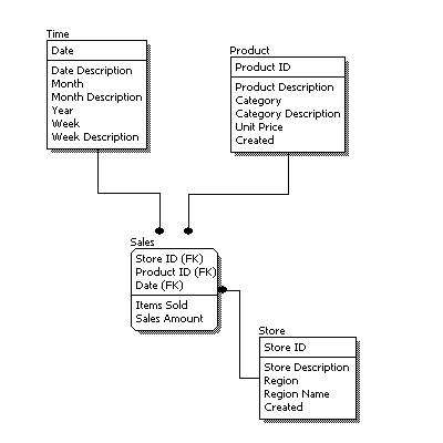
  • Explain Physical Data Model or PDM ?

Physical data model represents how the model will be built in the database. A physical database model shows all table structures, including column name, column data type, column constraints, primary key, foreign key, and relationships between tables. Features of a physical data model include:

  1. Specification all tables and columns.
  2. Foreign keys are used to identify relationships between tables.
  3. Specying Data types.

EG –

Reference from Here

  •  Explain Logical Data Model ?

A logical data model describes the data in as much detail as possible, without regard to how they will be physical implemented in the database. Features of a logical data model include:

  1. Includes all entities and relationships among them.
  2. All attributes for each entity are specified.
  3. The primary key for each entity is specified.
  4. Foreign keys (keys identifying the relationship between different entities) are specified.
  5. Normalization occurs at this level.

Reference from Here

  • Explain Conceptual Data Model ?

A conceptual data model identifies the highest-level relationships between the different entities. Features of conceptual data model include:

  1. Includes the important entities and the relationships among them.
  2. No attribute is specified.
  3. No primary key is specified.
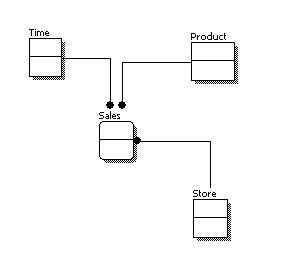
Reference from Here

  • What is Log Shipping ?

Log Shipping is a basic level SQL Server high-availability technology that is part of SQL Server. It is an automated backup/restore process that allows you to create another copy of your database for failover.

Log shipping involves copying a database backup and subsequent transaction log backups from the primary (source) server and restoring the database and transaction log backups on one or more secondary (Stand By / Destination) servers. The Target Database is in a standby or no-recovery mode on the secondary server(s) which allows subsequent transaction logs to be backed up on the primary and shipped (or copied) to the secondary servers and then applied (restored) there.

  •  What are the advantages of database normalization ?

Benefits of normalizing the database are

  1. No need to restructure existing tables for new data.
  2. Reducing repetitive entries.
  3. Reducing required storage space
  4. Increased speed and flexibility of queries.
  •  What are Linked Servers  ?

 Linked servers are configured to enable the Database Engine to execute a Transact-SQL statement that includes tables in another instance of SQL Server, or another database product such as Oracle. Many types OLE DB data sources can be configured as linked servers, including Microsoft Access and Excel. Linked servers offer the following advantages:

  1. The ability to access data from outside of SQL Server.
  2. The ability to issue distributed queries, updates, commands, and transactions on heterogeneous data sources across the enterprise.
  3. The ability to address diverse data sources similarly.
  4. Can connect to MOLAP databases too.
  •  What is the Difference between the functions COUNT and COUNT_BIG ?
Both Count and Count_Big functions are used to count the number of rows in a table and the only difference is what it returns.
  1. Count returns INT datatype value where as Count_Big returns BIGINT datatype value.
  2. Count is used if the rows in a table are less where as Count_Big will be used when the numbenr of records are in millions or above.

Syntax –

  1. Count – Select count(*) from tablename
  2. Count_Big – Select Count_Big(*) from tablename
  •  How to insert values EXPLICITLY  to an Identity Column ? 
This has become a common question these days in interviews. Actually we cannot Pass values to Identity column and you will get the following error message when you try to pass value.
Msg 544, Level 16, State 1, Line 3
Cannot insert explicit value for identity column in table 'tablename' when IDENTITY_INSERT is set to OFF.
To pass an external value we can use the property IDENTITY_INSERT. PFB the sysntax of the same.
SET IDENTITY_INSERT <tablename> ON;
Write your Insert  statement here by passing external values to the IDENTITY column.
Once the data is inserted then remember to SET the property to OFF.
  • How to RENAME a table and column in SQL ?
We can rename a table or a column in SQL using the System stored procedure SP_RENAME. PFB the sample queries.
Table – EXEC sp_rename @objname = department, @newname = subdivision
Column – EXEC sp_rename @objname = ‘sales.order_no’ , @newname = ordernumber
  • How to rename a database ?
To rename a database please use the below syntax.
USE master;
GO
ALTER DATABASE databasename
Modify Name = newname ;
GO
  •  What is the use the UPDATE_STATISTICS command ?
UPDATE_STATISTICS updates the indexes on the tables when there is large processing of data. If we do a large amount of deletions any modification or Bulk Copy into the tables, we need to basically update the indexes to take these changes into account.
  • How to read the last record from a table with Identity Column ?
We can get the same using couple of ways and PFB the same.
First – 
SELECT *
FROM    TABLE
WHERE  ID = IDENT_CURRENT(‘TABLE’)
Second – 
SELECT *
FROM    TABLE
WHERE   ID = (SELECT MAX(ID)  FROM TABLE)
Third – 
select top 1 * from TABLE_NAME  order by ID desc
  • What is Worktable ?

A worktable is a temporary table used internally by SQL Server to process the intermediate results of a query. Worktables are created in the tempdb database and are dropped automatically after query execution. Thease table cannot be seen as these are created while a query executing and dropped immediately after the execution of the query.

  • What is HEAP table ?

A table with NO CLUSTERED INDEXES is called as HEAP table. The data rows of a heap table are not stored in any particular order or linked to the adjacent pages in the table. This unorganized structure of the heap table usually increases the overhead of accessing a large heap table, when compared to accessing a large nonheap table (a table with clustered index). So, prefer not to go with HEAP  tables .. 🙂

  • What is ROW LOCATOR ?

If you define a NON CLUSTERED index on a table then the index row of a nonclustered index contains a pointer to the corresponding data row of the table. This pointer is called a row locator. The value of the row locator depends on whether the data pages are stored in a heap or are clustered. For a nonclustered index, the row locator is a pointer to the data row. For a table with a clustered index, the row locator is the clustered index key value.

  •  What is Covering Index ?

A covering index is a nonclustered index built upon all the columns required to satisfy a SQL query without going to the base table. If a query encounters an index and does not need to refer to the underlying data table at all, then the index can be considered a covering index.  For Example

Select col1,col2 from table
where col3 = Value
group by col4
order by col5

Now if you create a clustered index for all the columns used in Select statement then the SQL doesn’t need to go to base tables as everything required are available in index pages.

  •  What is Indexed View ?
A database view in SQL Server is like a virtual table that represents the output of a SELECT statement. A view is created using the CREATE VIEW statement, and it can be queried exactly like a table. In general, a view doesn’t store any data—only the SELECT statement associated with it. Every time a view is queried, it further queries the underlying tables by executing its associated SELECT statement.
A database view can be materialized on the disk by creating a unique clustered index on the view. Such a view is referred to as an indexed view. After a unique clustered index is created on the view, the view’s result set is materialized immediately and persisted in physical storage in the database, saving the overhead of performing costly operations during query execution. After the view is materialized, multiple nonclustered indexes can be created on the indexed view.
  • What is Bookmark Lookup ?

When a SQL query requests a small number of rows, the optimizer can use the nonclustered index, if available, on the column(s) in the WHERE clause to retrieve the data. If the query refers to columns that are not part of the nonclustered index used to retrieve the data, then navigation is required from the index row to the corresponding data row in the table to access these columns.This operation is called a bookmark lookup.

How to disable Reporting Services data cache in Development

249

Friends,

Microsoft provided data caching option which is a real great boon to the developers and few times the real curse too. Let me explain both the cases here.

Let’s say we have written a query which returns 1 million records from database and using the same output a SSRS report is designed. As you all know it takes minutes to get 1 million records from database and more time to display the same in SSRS report. The data is tested and it is perfectly working and not the work is on Look and Feel of the report like setting colors, fonts and more. When ever you make any change to the Format of the report then you have to see the preview of the report. Here comes the advantage of having data cache in SSRS designer. When ever I click on preview after making changes then the SSRS will uses the data cache option and displays the caches data with new format instead of hitting the database to fetch the data fresh. This helps us in saving our time while development. If this data cache option is not available then for every change the query will be hit and the data will be fetched from database. This will not have much impact if the query is fetching less data but when the data is huge then it is gonna kill the time during development. So, in simple when the report dataset is fetching huge data then better to have data cache enabled to save time during development.

Now, let’s see the disadvantages of having data cache  enabled. If the data is changed in your  database and you want to see it then this data cache should be disabled else it will pull and show the same old cached data again and again. Let me explain a scenario which killed my time. I was new to SSRS and when i was working on PROTOTYPE, I designed a report on DUMMY data and everything was working fine. When I have given demo to my manager he asked me to add more records before we give demo to user. I added more data and everything was set. When the demo to users started, we were surprised by seeing the same old junk data in report(including my name and my gf’s name .. :p). As I was not aware of this option it ruined my day. After long search in google I cam eotknow about this option.

So, it is very important to be aware of this option. This can be Enabled/Disabled in the file present in the below given folder.

C:\Program Files (x86)\Microsoft Visual Studio 9.0\Common7\IDE\PrivateAssemblies\RSReportDesigner.config

In that file you can see an option “CacheDataForPreview” and you have to turn this off/on to disable/enable this feature. PFB the screenshot showing the same.

This is a simple  feature but very useful one to developer. So, it is very useful to keep an eye on this while developing SSRS reports.

That’s it .. Hope you understood.

Regards,

Roopesh Babu V


Role Playing Dimensions in SSAS

52

Friends,

I am backkkk .. Long gap between my last post and this .. Here, in this post we are gonna discuss about ROLE PLAYING DIMENSIONS. I am gonna take same old and our favorite database “Adventure Works” to explain about Role Playing Dimensions. Lets say I have a scenario i.e I wish to see the sales happened based on Due dates,Ship Dates and Order Dates.These three dates MAY BE SAME and also MAY NOT BE as in many cases the ORDER will be given on one date and Shipment will be done on some other date and Dues will be paid on another date and hence this is very important for any Analyst to see the data based on different date types to get better idea about business. In this case I have to maintain THREE DATE KEY columns in my Fact table ONE for EACH date type given above. If you see the Fact table in Adventure Works database, it is designed in the same fashion.  I ran the query to fetch data from FactInternetSales table for the above given columns.

Select Top 100 OrderDateKey,ShipDateKey,DueDateKey,SalesAmount from FactInternetSales

From the above screenshot it is clear that Due Date,Order Date and Ship Date need not to be fall on same dates and hence we maintain different columns for each to track the status. Now, I wish to see the Total Shipment sales year wise. To get this I need to join the Fact table with Time table and the query looks like below.

Select DimTime.CalendarYear,Sum(SalesAmount) SalesAmount from FactInternetSales
Inner Join DimTime on DimTime.TimeKey = FactInternetSales.ShipDateKey
Group By DimTime.CalendarYear

In the above query I joined fact table (FactInternetSales) with Time table(DimTime) with SHIPDATEKEY as I wish to see the Sales year wise based on Shipments and the output can be seen in the screenshot given below.

Now, I wish to see the Total sales year wise based on ORDERED date. To get this I need to join the Fact table with Time table and the query looks like below.

Select DimTime.CalendarYear,Sum(SalesAmount) SalesAmount from FactInternetSales
Inner Join DimTime on DimTime.TimeKey = FactInternetSales.OrderDateKey
Group By DimTime.CalendarYear

In the above query I joined fact table (FactInternetSales) with Time table(DimTime) with ORDERDATEKEY as I wish to see the Sales year wise based on ORDER Date and the output can be seen in the screenshot given below.

And the final scenario i.e Sales year wise based on Due Date and the query looks like below.

Select DimTime.CalendarYear,Sum(SalesAmount) SalesAmount from FactInternetSales
Inner Join DimTime on DimTime.TimeKey = FactInternetSales.DueDateKey
Group By DimTime.CalendarYear

The output of the above query can be seen in the below screenshot.

From the above three results, it is obvious that the SALES VALUES doesn’t match as the transactions happened on different dates for each type. In OLTP database scenario, DIMTIME in the above query is referred as MASTER Table(where we will have master data of each entity) and FACTINTERNETSALES is referred as TRANSACTION table where we capture all transactions. In OLAP, we call DIMTIME as a Dimension and FACTINTERNETSALES as MEASUREGROUP or FACT.

Okie .. If the requirement is either one of the above mentioned three scenarios then NO ISSUES. We can create a Dimension using DimTime table, MeasureGroup using FactInternetSales table and give relationship between these two. What the Case if the user want to see the data based on all the three date types. Then the SQL query looks like some thing like given below.

Select a.CalendarYear,Sum(SalesAmount) SalesAmount from FactInternetSales
Inner Join DimTime a on a.TimeKey = FactInternetSales.DueDateKey
Inner Join DimTime b on b.TimeKey = FactInternetSales.OrderDateKey
Inner Join DimTime c on c.TimeKey = FactInternetSales.ShipDateKey
Group By a.CalendarYear

Even though the Date Types are different, the master data for all these are JUST Dates and hence ONLY ONE master table will be maintained. So, we have to use ALIAS of same DIMTIME table to join with different date types as shown above. The Group by and the Select list has a column “a.CalendarYear” and hence the data will be GROUPED yearwise based on DUE DATE as the alias “a” is joined with fact table with DueDateKey. To get the Sales Data year wise based on Order Date we simply need to change the Group By and Select list item a.CalendarYear to b.CalendarYear and to c.CalendarYear to get data based on Ship Date.

The same thing can be handled in SSAS Cubes using ROLE PLAYING DIMENSIONS property. PFB the Steps to define the same.

1) Add the fact table and the Dimension table to DSV as shown below and make sure RELATIONS are given for three date keys in Fact table to DimTime table.

2) Define dimension using DimTime table.

3) Create an Empty cube and add the Measure Group with FactInternetSales table.

4) Now add the dimension to the cube and see the magic. When you add one dimension, it adds THREE one for EACH date type. This is created based on the relationships given in DSV. I have THREE relations between DimTime and FactInterNetSales tables and hence THREE Dimension added. If you remove one relation ship in DSV and when you try to add the same dimension then it will add ONLY TWO dimensions. So, SSAS server will takes the headache of adding ALIAS Dimensions for each relationship given in DSV between these two tables.

Even though THREE ALIAS dimensions are created at Cube level, all the three will be pointing to the same underlying dimension as shown in below screenshot.

In the Dimension Usage tab the relations ships will be automatically set to the corresponding columns i.e ShipdateKey for Ship Date Dimension and so on as shown below.

So, the headache of creating ALIAS dimensions and giving relationships will be taken by SSAS Server if and only if the relationships are given in DSV between these tables. Now, what the case if the relationships are not given in SSAS( a rare case that happens). In this case all the headache will be on Developers who is developing the cube.

The steps remains the same as discussed above until Step 3. PFB the steps to be followed after completing the above given first three steps.

1) Add the dimension to the Cube and rename it to SHIP DATE.

2) Add the same dimension again and rename it to DUE DATE.

3) Add the same dimension again and rename it to ORDER DATE.

4) Go to Dimension Usage tab and click on the cell of each intersecting point and select the relationship type as REGULAR in the pop up wizard and select the columns to link. In the below screenshot I selected DueDateKey under MEasure Group Columns as I am relation DUE DATE Dimension to Fact table. Similarly we have to use OrderDateKey and ShipDateKey for Measure Group Columns to link with ORDER DATE Dimension and SHIP DATE Dimension respectively.

After adding relationships for all the three dimension PROCESS the cube and validate data by browsing cube. In simple Role Playing Dimension is a dimension which will have only ONE in database level and act as many DIMENSIONS in Cube.

That’s it .. Hope you guys understood the concept. Happy Coding !!

Regards,

Roopesh Babu V


How to Define/Implement Type 2 SCD in SSIS using Slowly Changing Dimension Transformation

1281

Friends,

In last post we discussed about “Implementing Type 1 SCD in SSIS using Slowly Changing Dimension Transformation” and u can find the same here. Let us discuss about “How to define Type 2 SCD in SSIS using Slowly Changing Dimension Transformation” in this post. As most of us know that there are many types of SCDS available, here in this post we will cover only SCD Type 2. Before jumping into the demonstration, first let us know what this SCD Type 2 says –

In Type 2 SCD, a new record is added to the table to represent the new information. Therefore, both the original and the new record will be present. The new record gets its own primary key.


Emp_ID Emp_Name Country Start_Date End_Date
1 Roopesh India 01-01-11 NULL

Now, when the Country is changed to the Employee “Roopesh” from India to USA then  the data will be stored in the following way –

Emp_ID Emp_Name Country Start_Date End_Date
1 Roopesh India 01-01-11 13-03-12
2 Roopesh USA 13-03-12 NULL

The null End_Date in row two indicates the current tuple version. In some cases, a standardized surrogate high date (e.g. 9999-12-31) may be used as an end date, so that the field can be included in an index, and so that null-value substitution is not required when querying. So, in this case we can say the records with NULL as End_Date is the current record for an employee.

The major disadvantage of using this is the table SIZE grows faster as records will get added whenever there is change in data to maintain history and the advantage of using this Type is that we can track historical information accurately.  I hope you got some useful info regarding SCD type 2 and now let’s jump into SCD Transformation.

I have created two tables one Test_Stage(Which I am using as Staging table) and another one is Test(Which I am using as Main table) with the following syntax. You can clearly see that Main table is having TWO Extra columns to track history.

Create table Test_Stage
(
Emp_Id int,
Emp_Name Varchar(100),
Country Varchar(100)
)

Create table Test
(
Emp_Id int,
Emp_Name Varchar(100),
Country Varchar(100),
Start_Date Datetime,
End_Date DateTime
)

Now I inserted some records into my staging table i.e Test_Stage and PFB the scripts used –

Insert into test_stage Values(1,’Roopesh’,’India’);
Insert into test_stage Values(2,’Lokesh’,’Pakistan’);
Insert into test_stage Values(3,’Vinay’,’USA’);
Insert into test_stage Values(4,’Rakesh’,’China’);
Insert into test_stage Values(5,’Venki’,’Japan’);

Now Source data is ready and PFB the steps you have to follow to use Slowly Changing Dimension Transformation to implement Type 2 SCD.

  • Open SSIS Package and drag a dataFlow Task from toolbox to control Flow Pane as shown below.
  • Either double click or Right click on Data Flow Task and select EDIT as shown below.
  • One the Data Flow pane is opened then drag and drop OLEDB SOURCE from “Data Flow Sources” as shown below.
  • Now select EDIT by Right clicking on OLE DB Source and provide the Source details. remember that you have to provide Staging table connection details here.
  • Select columns tab and check whether columns are coming correctly or not.

  • Now drag and drop Slowly Changing Dimension Transformation in to the Data Flow Pane and provide the connection between OLE DB Source and SCD Transformation.
  • Now right click on the SCD Transformation and click on EDIT menu.
  • Select the dimension table(in our case it is “Test”) and Keys under “Select Dimension Table and Keys” page as shown below.

  • In the above screenshot, the Business Key is the column based on which we will filter the Newly added records from the existing one. In simple this is the column which we use to look up.
  • After selecting Next, Under “Slowly Changing Dimension Columns” select the columns that MAY change and select Change Type as “Changing Attribute” for those which we DOESN’T required to maintain HISTORY and select “Historical Attribute” for those whose HISTORY needs to be tracked. This is very important part of SCD and in other words this is the ONLY change we have when compared to SCD Type 1 and SCD Type 2 implementation in SSIS. When we select “Changing Attribute” for any attribute then it WON’T CREATE a new record when there is a change in this value and if you select “Historical Attribute” then if there is any change in this attribute value then a NEW RECORD will be created to track history.
  • In the above screenshot we can see that for Country attribute I selected “Historical Attribute” as I wish to track the historical changes for that attribute and hence when ever there is a change in that particular attribute column value then only it tracks history by creating a new record and for other attribute Emp_Name, it will directly apply UPDATE on the table.


  • Check the option “Change all the matching records including the outdated records…….” if you wish to have that functionality and click Next.
  • Under “Historical Attributes Option” page select “Use Start and End date to identify current and expired records” option and by selecting start date column and End date column click on NEXT.
  • Click Next and finally click on Finish by leaving the default options as is.
  • Once you click on Finish, SSIS server creates all the functionality that is required to implement SCD Type 1 based on the information provided by us. It will add Data flow tasks for Inserting new records and updating existing records as shown below.
  • Now if I run the package then it will check for newly added records and inserts those records and updates the already existing records if there is any change in data. As there is NO RECORDS in TEST table in this run it will load all the records under New Insert as shown below.
  • PFB the Screenshot of the data tables output after running the package. You can see data got loaded in to our table “TEST” with Start_Date as current Date.
  • Now I updated the existing records in staging table using the following queries and once I run the package again we can see data getting updated into our main table.
              update test_stage set Country = ‘USA’ where Emp_Id = 1
  • Once I run the package you can see the package showing “1 rows” under “Historical Attributes Inserts Output” section as shown below.
  • Now if you run the queries you can see the data updated in TEST table.
That’s it guys .. Now we implemented SCD Type 2 using Slowly Changing Dimension Transformation. This is as simple as this. Hope you understood the concept. Happy Coding !!

Regards,

Roopesh Babu V

How to Define/Implement Type 1 SCD in SSIS using Slowly Changing Dimension Transformation

572

Friends,

Let us discuss about “How to define Type 1 SCD in SSIS using Slowly Changing Dimension Transformation” in this post. As most of us know that there are many types of SCDS available, here in this post we will cover only SCD Type 1. Before jumping into the demonstration, first let us know what this SCD Type 1 says –

In Type 1 SCD we will overwrite the existing data with the new data. Lets take a small example here. Lets say I have data like given below in my existing table.

Emp Key Name Country
1 Roopesh India

Let’s say the employee is not moved to USA from India. Now, the data that is present in the database table will be directly replaced with the new data and we will have the following data in table.

Emp Key Name Country
1 Roopesh USA

The major disadvantage of using this method is HISTORY will be lost. If we implement this methodology then we can’t track the history of a particular employee. So, this is not at all suggestible in the case where HISTORY needs to be maintained.

This is the easiest way to implement of all th SCD types available. So, Type 1 slowly changing dimension should be used when it is NOT NECESSARY for the data warehouse to keep track of historical changes. I hope you got some useful info regarding SCD type 1 and now let’s jump into SCD Transformation.

I have created two tables one Test_Stage(Which I am using as Staging table) and another one is Test(Which I am using as Main table) with the following syntax.

Create table Test_Stage
(
Emp_Id int,
Emp_Name Varchar(100),
Country Varchar(100)
)

Create table Test
(
Emp_Id int,
Emp_Name Varchar(100),
Country Varchar(100)
)

Now I inserted some records into my staging table i.e Test_Stage and PFB the scripts used –

Insert into test_stage Values(1,’Roopesh’,’India’);
Insert into test_stage Values(2,’Lokesh’,’Pakistan’);
Insert into test_stage Values(3,’Vinay’,’USA’);
Insert into test_stage Values(4,’Rakesh’,’China’);
Insert into test_stage Values(5,’Venki’,’Japan’);

Now Source data is ready and PFB the steps you have to follow to use Slowly Changing Dimension Transformation.

  • Open SSIS Package and drag a dataFlow Task from toolbox to control Flow Pane as shown below.
  • Either double click or Right click on Data Flow Task and select EDIT as shown below.
  • One the Data Flow pane is opened then drag and drop OLEDB SOURCE from “Data Flow Sources” as shown below.
  • Now select EDIT by Right clicking on OLE DB Source and provide the Source details. remember that you have to provide Staging table connection details here.
  • Select columns tab and check whether columns are coming correctly or not.

  • Now drag and drop Slowly Changing Dimension Transformation in to the Data Flow Pane and provide the connection between OLE DB Source and SCD Transformation.
  • Now right click on the SCD Transformation and click on EDIT menu.
  • Select the dimension table(in our case it is “Test”) and Keys under “Select Dimension Table and Keys” page as shown below.

  • In the above screenshot, the Business Key is the column based on which we will filter the Newly added records from the existing one. In simple this is the column which we use to look up.
  • After selecting Next, Under “Slowly Changing Dimension Columns” select the columns that MAY change and select Change Type as “Changing Attribute” as we are dealing with Type 1 SCD here. Once the selection is done the click on NEXT.

  • Check the option “Change all the matching records including the outdated records…….” if you wish to have that functionality and click Next.

  • Click Next and finally click on Finish by leaving the default options as is.
  • Once you click on Finish, SSIS server creates all the functionality that is required to implement SCD Type 1 based on the information provided by us. It will add Data flow tasks for Inserting new records and updating existing records as shown below.

  • Now if I run the package then it will check for newly added records and inserts those records and updates the already existing records if there is any change in data. As there is NO RECORDS in TEST table in this run it will load all the records under New Insert as shown below.

  • PFB the Screenshot of the data tables output before running the package and After running it. You can see data got loaded in to our table “TEST”.

  • Now I updated the existing records in staging table using the following queries and once I run the package again we can see data getting updated into our main table.

update test_stage set Country = ‘USA’ where Emp_Id = 1

  • Once I run the package you can see the package showing “1 rows” under “Changing Attributes Updates Output” section as shown below.

  • Now if you run the queries you can see the data updated in TEST table.

That’s it guys .. Now we implemented SCD Type 1 using Slowly Changing Dimension Transformation. This is as simple as this. Hopw you understood the concept. Happy Coding !!

Regards,

Roopesh Babu V


Mean and Median in SSRS Reports

724

Friends,

Let us discuss about “How to show MEAN and MEDIAN” of a series in a chart in this post. This post is specially for those who doesn’t know that there is an option available in SSRS to show MEAN and MEDIAN in reports. To demonstrate the same lets us take a simple query from Adventure Works database. This query pulls Product wise sales from the database. PFB the query –

SELECT Top 30 DimProduct.EnglishProductName, SUM(FactInternetSales.SalesAmount) AS Sales
FROM FactInternetSales INNER JOIN
DimProduct ON DimProduct.ProductKey = FactInternetSales.ProductKey
GROUP BY DimProduct.EnglishProductName

To make the report look better, I am pulling ONLY top 30 records from the database.

Now create a “Dataset” in SSRS report using the above query.

Now take a line chart from ToolBox and drag and drop EnglishProductName to “Category Fields” and Sales to “Data Fields” of Line chart as shown in below pic.

Now Right click on “Sales” which is added to “Data Fields” and select “Add Calculated Series” option.

Select “Mean” from the dropdownlist next to label “Formula” and select OK.

Repeat the last TWO steps and add MEDIAN to the Line chart. Now click on PREVIEW to preview your report. You can see MEAN and MEDIAN series added to your chart.

That’s it .. It is as simple as this. Hope you understood and Happy coding !!

Regards,

Roopesh Babu V

Tracking Report usage in SSRS Reports

127

Friends,

We all know about our managers, they are like piles, both wont allow us to sit peacefully for 10 mins. I worked under many managers and not even one allowed me to take rest when I don’t have any work. One guy given me a shit work i.e “Finding out the usage of reports deployed in server”.

If we jump into story, We worked hard day and night and deployed reports in server after proper testing. So, few days no work and once day manager called me and asked me to give the usage of EACH report in server. I asked Why and for that he replied because WE both doesn’t have any work.

After some goggling I found a way to get that report in one shot and I am sharing the same for you guys. All the report related information will be stored in “ExecutionLog” table in “Report Server” Database. PFB the query that pulls the Report usage information of SSRS Reports.

SELECT
UserName, Format, TimeStart, Name,
Parameters,
CONVERT(nvarchar(10), TimeStart, 101) AS rundate
FROM ExecutionLog, Catalog
where ReportID = Catalog.ItemID
ORDER BY TimeStart DESC

If you wish to see how many times a report was run then you can use the below code

SELECT
Name,
COUNT(*)
FROM ExecutionLog, Catalog
where ReportID = Catalog.ItemID
Group by Name

Hope this will help you guys .. Happy Coding !!

Regards,

Roopesh Babu V

YTD – “By Default, a year level was expected. No such level was found in the cube” Error in MDX

275

Friends,

“By Default, a year level was expected. No such level was found in the cube” is the most common error in MDX when a newbie in MDX is using YTD function. YTD is one of very powerful functions provided my Microsoft in MDX. YTD gives YEAR to DATE value of the measure passed. PFB the syntax of YTD function.

YTD(Member_Exp)

Member_Exp – Valid Member Expression which returns a member from TIME Dimension Hierarchy.

For example if I pass Nov 2011 as a member to the YTD function then it calculates the sum of measure value from Jan 2011 to Nov 2011 and provide you the result. PFB a sample query which shows how to use YTD fucntion.

SUM(YTD(Member_Exp),Measure).

Let’s discuss about the most common error we get when we use YTD function i.e “By Default, a year level was expected. No such level was found in the cube”. When I started my career in SSAS and MDX I tried a lot to solve this issue and make YTD function work. I failed to and used alternate function PERIODSTODATE which helps in achieving the output required. Let’s take a sample query which has YTD function in it.

With member [Measures].[YTD] as
SUM(YTD([Dim Time].[Hierarchy].CurrentMember),[Measures].[Sales Amount])
Select {[Measures].[Sales Amount],[Measures].[YTD]} on Columns,
[Dim Time].[Hierarchy].[Calendar Quarter] on Rows
From [Adventure Works]

If you see the above query the YTD function calculates the Year to Date of Sales Amount based on Current ROW item but if you see the above screenshot it is throwing error “By Default, a year level was expected. No such level was found in the cube”. The reason for this error is the definition of your time dimension.

When ever you are using the functions like YTD,MTD,WTD and QTD then you have to make sure of the following things.

  • Dimension Type of the dimension from where you are passing member_exp to YTD function should be of TYPE TIME.
  • Calendar related Type should be set to the attributes used in the Hierarchy.

Let’s see how to change the Type of Dimension and Attributes and make this YTD function work.

  • Select the dimension and press F4 for properties window. In properties window change the Type to TIME as shown below.
  • Now select Calendar Year attribute and go to properties. Select “Years” under “Calendar Year” which is under “Date” item as show in below screenshot.
  •  Repeat the above step for the remaining attributes which are used as part of Hierarchy. Select Quarters,Months,Weeks .. from the list under Attribute type just like we selected “Years” in last step.
  • Once all the Types for attributes are selected then process the cube and run the same query which failed for YTD earlier. Yoc can see YTD getting calculated.

That’s it .. Hope you understood how to solve this issue and Happy Coding !!

Regards,

Roopesh Babu V

How to browse cube in Excel

595

Friends,

We have soooo many tools to browse cube data. We can use MDX to pull data from SSAS cube and use the result set to generate reports using many tools like ssrs,dundas,xmla .. There are many tools like this but Client’s most favorite  and even green to browse cube is EXCEL. In this post we are gonna see how to connect to SSAS Cube from Excel. I have a cube ready in my server for this demonstration. PFB the steps to be followed:

  • Open Excel Sheet.
  • Select DATA tab on top of the sheet.
  • Select “From Analysis Services” under “From Other Sources” tab as shown below.

  • Provide the server name and the authentication details and click on next. In my case the server is my local computer and hence given as LOCALHOST as shown below.

  • Select cube database name from drop down list and click on next by selecting the cube as shown below.

  • Click on Finish. I will ask you to select the way you wish to IMPORT DATA. Leave the settings as is and click on OK. This will create a Pivot Table Report in Excel sheet.

  • You c an see Pivot Table Area on the left hand side of the sheet and Field list from cube on the right hand side of the sheet. You can drag and drop fields into ROWS,COLUMNS,FILTERS and VALUES to see the desired report as shown below.

That’s it .. You can play with Pivot by dragging and dropping Attributes and Measures on the required pane. Hope you understood it .. Happy coding !!

Regards,

Roopesh Babu V

Custom Code in SSRS

266

Friends,

SSRS is a very good reporting tool and the only problem with this is This is a LIMITED one I feel. Limited in the sense, that the functions you can use is limited and hence it may not help you to acheive all the requirements of the clients. When the customer’s requirement exceeds the capability of Built-in functions of SSRS then we will need to write own own Code to meet the requirements. Writing your own code(function) is called Custom Code and this is a very useful feature provided by Microsoft. In this article I will demonstrate how to add custom code to SSRS.

There are two ways in which you can write your custom functions and use it in your report.

  • Writing Code inside the report
  • Using Custom Assemblies

Let us discuss about the first option here:

Let’s say we have to design a function which returns the Status of the sales of each product. For that lets create a report first which displays Product and Sales Amount as shown in the below pic –

  • Select “Report Properties” from Reports main menu or in design View Right Click the design surface outside the border of the report and select “Report Properties” as shown below.

  • Select Code tab and paste the following code to create custom function

Public Function Test(ByVal Sales As Decimal) As String
Dim status As String
If Sales >= 2000 Then
status = “High Profit”
ElseIf Sales >= 500 Then
status = “Moderate Profit”
Else
status = “Low Profit”
End If
Return status
End Function

  • Click OK and now add a column to the Table used in report and give header as “Status” and right click on the data sell and select Expression as shown below.

  • Write the expression as shown below and select OK.

=Code.Test(Fields!SalesAmount.Value) — “Fields!SalesAmount.Value” field based on which you wish to calculate status.

  • Your report with Custom Funcmtion to calculate the Status(in other words KPI) is ready and if you click on preview you can see the output of the function you created.

That’s it .. Let us discuss about the second option in next post. Hope you understood how to add your custom code and make use of it in your report. Happy Coding !!

Regards,

Roopesh Babu V

Parameters using Stored Procedures in SSRS Reports

615

Friends,

Here in this post we are gonna discuss about how to use SP(Stored Procedures) to get input for Parameters in SSRS Reports. If you wish to define parameters using Sql Queries then you can find the sample here. For this demonstration purpose I Created three Stored procedures with the following names –

  • sp_getcategories – To pull categories
  • sp_getsubcategories – To pull Subcategories
  • sp_getProducts – To pull products

All the above three SPS are pretty straigh forward and you can find code below.

Create procedure sp_getCategories
as
select ProductCategoryKey,EnglishProductCategoryName as “Categories” from dimproductcategory
Go

Create procedure sp_getSubCategories @CatID int
as
select ProductSubCategoryKey,EnglishProductSubCategoryName as “SubCategories” from dimproductsubcategory
Where ProductCategoryKey = @CatID
Go

Create procedure sp_getProducts @SubCatID int
as
select ProductKey,EnglishProductName as “Products” from dimproduct
Where ProductSubCategoryKey = @SubCatID

If you see the code for all the three SPS, the first one has no parameter and it pulls all the Categories. The second one pulls Subcategory names based on the CategoryKey we pass. The third one pulls Products info based on the SubcategoryKey we pass. PFB the screenshot showing the result set of the SPS.

Now lets design a report with THREE parameters which pulls data using SPS. First I created a report(Tabular) using the following query –

SELECT DimProductCategory.EnglishProductCategoryName, DimProductSubcategory.EnglishProductSubcategoryName, DimProduct.EnglishProductName, FactInternetSales.SalesAmount, FactInternetSales.TotalProductCost, FactInternetSales.TaxAmt, FactInternetSales.Freight FROM DimProduct INNER JOIN DimProductSubcategory ON DimProduct.ProductSubcategoryKey = DimProductSubcategory.ProductSubcategoryKey INNER JOIN DimProductCategory ON DimProductSubcategory.ProductCategoryKey = DimProductCategory.ProductCategoryKey INNER JOIN
FactInternetSales ON DimProduct.ProductKey = FactInternetSales.ProductKey

and pfb the report screenshot.

At this point of time there are no Parameters defined and hence you will get all the data from the database and will be displayed in the report. PFB the steps to be followed to ADD PARAMETERS to your report using SPS as source –

  • Right click on Datasource and select “Add Dataset” option.
  • Select the data source and select the option “Stored Procedure” radio button and provide the Stored Procedure name which pulls values for parameter and as I am adding “Category” as parameter I am using the following stored procedure which pulls Categories data.

  • As there is no INPUT parameters for this Stored Procedure we can continue by Clicking OK. When you click on OK , you can see new data set added with TWO columns as shown in below screenshot.
  • Now Right Click on “Parameters” and select “Add Parameters” option. The wizard will get open and Chnage the default value given for NAME and PROMPT if required.

  • Now select the “Available Values” tab which is on the Left hand side of the wizard and select the option “Get Values From a Query”. Provide the Dataset name,Value Field and Label Field as shown below –
  • Click on OK and with this our First parameter using SP is added to report.
  • As the remaining SPS has input parameters, the creation of those slightly changes when compared to the last one. Let’s create the parameters using SP and having input parameters to SP.
  • Right click on Datasource and select “Add Dataset” option.
  • Select the data source and select the option “Stored Procedure” and provide the SP name which pulls values for parameter.
  • The above SP has a Input Parameter and hence to provide input value to the parameter select PARAMETERS tab and provide the Parameter value as shown below.

  • When you click on OK by providing the query, you can see new data set added with TWO columns which we can use to define the second parameter.
  • Right click on “Parameters” and select “Add New Parameter”.
  • When the wizard opens, Change the Prompt and Name if you wish to provide proper names.
  • Go to the “Available Values” tab and select the option “Get Values from Query” and select the values as shown below.

  • Select OK and repeat the same for the remaining parameter “Products” also.
  • Now all the report parameters are ready. Here the sequence of parameters are as follows – Category –> Sub Category–> Product and you can see the same in the below given screenshot.

  • If you see the above screenshot the  Parameters looks like working fine i.e when u Sub Category is listing only those records which belongs to the category selected and the same for Products too but if you see the chart area the data doesn’t look correct. This is because we added parameters but not linked those parameters to the Main dataset from which we are getting data and filling the chart. Now I will modify the Main dataset in order to fetch data by applying parameter values. Edit the main dataset and update the query as shown below –

SELECT DimProductCategory.EnglishProductCategoryName, DimProductSubcategory.EnglishProductSubcategoryName, DimProduct.EnglishProductName,FactInternetSales.SalesAmount, FactInternetSales.TotalProductCost, FactInternetSales.TaxAmt, FactInternetSales.Freight FROM DimProduct INNER JOIN DimProductSubcategory ON DimProduct.ProductSubcategoryKey = DimProductSubcategory.ProductSubcategoryKey INNER JOIN DimProductCategory ON DimProductSubcategory.ProductCategoryKey = DimProductCategory.ProductCategoryKey INNER JOIN FactInternetSales ON DimProduct.ProductKey = FactInternetSales.ProductKey Where DimProduct.ProductKey = @ReportParameter3 and DimProductSubCategory.ProductSubCategoryKey = @ReportParameter2 and DimProductCategory.ProductCategoryKey = @ReportParameter1

  • Now Select Parameters tab and map the parameters as shown below.

  • Click on OK and your report is ready. Go to preview tab and test you report. You can see Parameters cascading and the Report data get filtered as shown below –

That’s it .. Your Report with Parameters which is sourced from Stored Procedures is Ready .. Hope you understood the concepts .. Happy Coding !!

Regards,

Roopesh Babu V

Multi Valued Parameters in SSRS

253

Friends,

We discussed a lot about Singled Valued parameters here. Please fo through that post before jumping into this. If the user can select only one value from the parameter list then that is called Single Valued Parameters and if the user is able to select More than one then we call it as Multi Valued Parameters. First, Let us see how to add a Single Valued parameter to the report and then convert it to Multi Valued one. So, let’s jump into the topic –

First I created a report(Tabular) using the following query –

SELECT DimProductCategory.EnglishProductCategoryName, DimProductSubcategory.EnglishProductSubcategoryName, DimProduct.EnglishProductName, FactInternetSales.SalesAmount, FactInternetSales.TotalProductCost, FactInternetSales.TaxAmt, FactInternetSales.Freight FROM DimProduct INNER JOIN DimProductSubcategory ON DimProduct.ProductSubcategoryKey = DimProductSubcategory.ProductSubcategoryKey INNER JOIN DimProductCategory ON DimProductSubcategory.ProductCategoryKey = DimProductCategory.ProductCategoryKey INNER JOIN
FactInternetSales ON DimProduct.ProductKey = FactInternetSales.ProductKey

At this point of time there are no Parameters defined and hence you will get all the data from the database and will be displayed in the report. PFB the steps to be followed to ADD PARAMETERS to your report –

  • Right click on Datasource and select “Add Dataset” option.
  • Select the data source and provide the query which pulls values for parameter and as I am adding “Products” as parameter I am using the following query.

select ProductKey,EnglishProductName as “Products” from dimproduct

  • When you click on OK by providing the query, you can see new data set added with TWO columns as shown in below screenshot.
  • Now Right Click on “Parameters” and select “Add Parameters” option. The wizard will get open and Chnage the default value given for NAME and PROMPT if required.

  • Now select the “Available Values” tab which is on the Left hand side of the wizard and select the option “Get Values From a Query”. Provide the Dataset name,Value Field and Label Field as shown below –

  • Click OK and then edit the MAIN DATASET to add this parameter to the query. For that double click on Main dataset “Dataset1” in this case and modify the query with the given one below.

SELECT DimProductCategory.EnglishProductCategoryName, DimProductSubcategory.EnglishProductSubcategoryName, DimProduct.EnglishProductName,
FactInternetSales.SalesAmount, FactInternetSales.TotalProductCost, FactInternetSales.TaxAmt, FactInternetSales.Freight
FROM DimProduct INNER JOIN
DimProductSubcategory ON DimProduct.ProductSubcategoryKey = DimProductSubcategory.ProductSubcategoryKey INNER JOIN
DimProductCategory ON DimProductSubcategory.ProductCategoryKey = DimProductCategory.ProductCategoryKey INNER JOIN
FactInternetSales ON DimProduct.ProductKey = FactInternetSales.ProductKey
Where DimProduct.ProductKey = @ReportParameter1

  • Now Select Parameters tab and map the parameters as shown below.

  • Click on OK and your report is ready. Go to preview tab and test you report. You can see Report data get filtered as shown below  but the problem is at a time ONLY ONE Value can be selected as parameter.

  • To make is a Multi-Valued parameter double click on the parameter and check the option “Allow Multiple Values” as shown below.

  • Now if you preview the report, it will let you select multiple values but on submit it will throw error and pfb screenshot of the same.
  • This is because we are passing MULTI VALUES to the query but the query condition is “=” which expects a scalar value. To solve this issue go to the Main dataset query and change the query as given below.

SELECT DimProductCategory.EnglishProductCategoryName, DimProductSubcategory.EnglishProductSubcategoryName, DimProduct.EnglishProductName,
FactInternetSales.SalesAmount, FactInternetSales.TotalProductCost, FactInternetSales.TaxAmt, FactInternetSales.Freight
FROM DimProduct INNER JOIN
DimProductSubcategory ON DimProduct.ProductSubcategoryKey = DimProductSubcategory.ProductSubcategoryKey INNER JOIN
DimProductCategory ON DimProductSubcategory.ProductCategoryKey = DimProductCategory.ProductCategoryKey INNER JOIN
FactInternetSales ON DimProduct.ProductKey = FactInternetSales.ProductKey
Where DimProduct.ProductKey in (@ReportParameter1)

  • Now preview the report by selecting multiple values and pfb the screenshot of my sample report output.

There it you .. The required output. For multiple parameters see the blog post Cascading parameters here.

That’s it .. Hope you understood .. Happy Coding !!

Regards,

Roopesh Babu V

Adding Cascading Parameters to SSRS Reports

61

Friends,

Parameters are used to specify the data to use in a report. There are two types of parameters in a report –

  • Query Parameters – When you define a dataset query that includes variables, Reporting Services creates corresponding query parameters. Query parameters are used to limit data retrieved from the data source to just the data needed for the report.
  • Report Parameters – Report parameters appear on the report toolbar and allow report readers to select or enter values that are used when a report is processed. In Report Designer, report parameters are created automatically from query parameters. In Report Builder, report parameters are created when you set a prompt on a filter clause. You can also define report parameters that are not tied to query parameters.

Now let’s see how to add Parameters to a Report. Here in this post we are gonna discuss about Single Valued Parameters and for that I selected OUR Adventure Works Database as Data source. First I created a report(Tabular) using the following query –

SELECT DimProductCategory.EnglishProductCategoryName, DimProductSubcategory.EnglishProductSubcategoryName, DimProduct.EnglishProductName, FactInternetSales.SalesAmount, FactInternetSales.TotalProductCost, FactInternetSales.TaxAmt, FactInternetSales.Freight FROM DimProduct INNER JOIN DimProductSubcategory ON DimProduct.ProductSubcategoryKey = DimProductSubcategory.ProductSubcategoryKey INNER JOIN DimProductCategory ON DimProductSubcategory.ProductCategoryKey = DimProductCategory.ProductCategoryKey INNER JOIN
FactInternetSales ON DimProduct.ProductKey = FactInternetSales.ProductKey

and pfb the report screenshot.

At this point of time there are no Parameters defined and hence you will get all the data from the database and will be displayed in the report. PFB the steps to be followed to ADD PARAMETERS to your report –

  • Right click on Datasource and select “Add Dataset” option.
  • Select the data source and provide the query which pulls values for parameter and as I am adding “Category” as parameter I am using the following query.
             select ProductCategoryKey,EnglishProductCategoryName as “Categories” from dimproductcategory.
  • When you click on OK by providing the query, you can see new data set added with TWO columns as shown in below screenshot.
  • Now Right Click on “Parameters” and select “Add Parameters” option. The wizard will get open and Chnage the default value given for NAME and PROMPT if required.
  • Now select the “Available Values” tab which is on the Left hand side of the wizard and select the option “Get Values From a Query”. Provide the Dataset name,Value Field and Label Field as shown below –
  • Click on OK and with this our First parameter is added to report.

As we are gonna design cascading parameters, the remaining parameters creation changes a bit as those are depended on other parameters and here let us see how to define the parameter for Sub Categories.

  • Right click on Datasource and select “Add Dataset” option.
  • Select the data source and provide the query which pulls values for parameter and as I am adding “Sub Category” as parameter I am using the following query.

select ProductSubCategoryKey,EnglishProductSubCategoryName as “SubCategories” from dimproductSubcategory
Where ProductCategoryKey = @ReportParameter1

  • The above query has a WHERE clause and @ReportParameter1 as varaible. This is because the values of SubCategory parameter is based on the selection of Categories parameter.
  • Now select parameters tab on left hand side and select the “Parameter Value” from the list of available parameters as shown below.
  • When you click on OK by providing the query, you can see new data set added with TWO columns as shown in below screenshot.
  • Right click on “Parameters” and select “Add New Parameter”.
  • When the wizard opens, Change the Prompt and Name if you wish to provide proper names.
  • Go to the “Available Values” tab and select the option “Get Values from Query” and select the values as shown below.
  • Select OK and you can see your first cascading parameter got created.
  • Now repeat the same step to create one more parameter “Products” whose value is depended on selection of “SubCategories” and PFB the query for the same.

select ProductKey,EnglishProductName as “Products” from dimproduct
Where ProductSubCategoryKey = @ReportParameter2

Now all the report parameters are ready. Here the sequence of parameters are as follows – Category –> Sub Category–> Product and you can see the same in the below given screenshot.

If you see the above screenshot the  Parameters looks like working fine i.e when u Sub Category is listing only those records which belongs to the category selected and the same for Products too but if you see the chart area the data doesn’t look correct. This is because we added parameters but not linked those parameters to the Main dataset from which we are getting data and filling the chart. Now I will modify the Main dataset in order to fetch data by applying parameter values. Edit the main dataset and update the query as shown below –

SELECT DimProductCategory.EnglishProductCategoryName, DimProductSubcategory.EnglishProductSubcategoryName, DimProduct.EnglishProductName,FactInternetSales.SalesAmount, FactInternetSales.TotalProductCost, FactInternetSales.TaxAmt, FactInternetSales.Freight FROM DimProduct INNER JOIN DimProductSubcategory ON DimProduct.ProductSubcategoryKey = DimProductSubcategory.ProductSubcategoryKey INNER JOIN DimProductCategory ON DimProductSubcategory.ProductCategoryKey = DimProductCategory.ProductCategoryKey INNER JOIN FactInternetSales ON DimProduct.ProductKey = FactInternetSales.ProductKey Where DimProduct.ProductKey = @ReportParameter3 and DimProductSubCategory.ProductSubCategoryKey = @ReportParameter2 and DimProductCategory.ProductCategoryKey = @ReportParameter1

Now Select Parameters tab and map the parameters as shown below.

Click on OK and your report is ready. Go to preview tab and test you report. You can see Parameters cascading and the Report data get filtered as shown below –

That’s it .. Your Report with Parameters is Ready .. Hope you understood the concepts .. Happy Coding !!

Regards,

Roopesh Babu V

Children Function in MDX

226

Friends,

This acts similar to AllMembers function when you use this with attributes. PFB sample query of using Children function with attribute.

select [Measures].[Sales Amount] on 0,
[Dim Product].[Products].children on 1
from [Adventure Works]

or

select [Measures].[Sales Amount] on 0,
[Dim Product].[Products].AllMembers on 1
from [Adventure Works]

Both the above queries gives the same output. The power of CHILDREN function will come into picture when you are using this function with Hierarchies. Children function returns the next level members of a specified member or simply to say it returns Children of a member. 

Syntax:

“Member_Expression.Children”

If you have a hierarchy defined then this Children function returns the naturally ordered set which is the children of the member specified. If the specified member has no children, this function returns an empty set.

To demonstrate Children function I created a Dimension named “Dim Time” and defined a Hierarchy with the following levels.

  • Calendar Year
  • Calendar Quarter
  • English Month Name

Now, in the below query I passed 2002 from “Calendar year” level as member_expression to the children function and the query returned the children of 2002 member i.e Quarters 1,2,3,and 4 as shown in below Screenshot.

select [Measures].[Sales Amount] on 0,
[Dim Time].[Hierarchy].[Calendar Year].&[2002].Children on 1
from [Adventure Works]

Now in the below Example I am passing Member from “English Month Name” level of the hierarchy and as this is the last level of the hierarchy, there won’t be any children and hence it returns empty result set as shown in the below screenshot.

select [Measures].[Sales Amount] on 0,
[Dim Time].[Hierarchy].[Calendar Year].&[2002].&[4].&[December].Children on 1
from [Adventure Works]

Note: It is not that the Result set will be empty when you take a member from LAST level of the hierarchy. When you pass ANY MEMBER from ANY LEVEL which doesn’t have children then the result set will be empty. This looks very simple one but it is very useful and powerful when working on MDX Calculations.

That’s it .. Happy Coding !!

Regards,

Roopesh Babu V


BottomSum Function in MDX

35

Friends,

This funcmtion is very much similary to the functions BottomCount and BottomPercent. Please find the Major Difference between the all three functions –

1) BottomCount – Orders the set and then returns specified number of tuples in the specified set with the lowest values will be pulled.

2) BottomPercent – Orders the set and then returns tuples from the bottom of the set with the lowest values whose cumulative total is less than or equal to the supplied percentage.

3) BottomSum – Orders the set and then returns the summed value of a numeric expression across a supplied set.

In this post we are gonna discuss about BottomSum Function. This function will do TWO jobs –

1) Sorts the set based on numeric parameter in Ascending order.

2)  Returns tuples from the bottom of the set with the lowest values whose cumulative total is less than or equal to the supplied Number.

Syntax –

BottomSum(Set_Exp,Value,Numeric_Exp)

Set_Exp – Valid MDX Set Expression

Value – It specifies the Total Value of Cumulative sum of records to be returned.

Numeric_Exp – It specifies on what column basis the set needs to be ordered.

The BottomSum function sorts a set in ascending order, then returns tuples from the bottom of the set with the lowest values whose cumulative total is less than or equal to the supplied value. This function returns the smallest subset of a set whose cumulative total is at least equal or near to the specified value. The returned elements are ordered largest to smallest.

PFB sample query Which pulls 10 Percent of Products based on Sales Amount.

select [Measures].[Sales Amount] on 0,
BottomSum([Dim Product].[Products].[Products],10000,[Measures].[Sales Amount]) on 1
from [Adventure Works]

If you see the above screenshot, the sum of returned values looks like more than the value specified and it is becausxe that the BOTTOMSUM function returns NEAREST value to the specified value in parameters. It is returning soo many records among which most are having NULL as Sales Amount. As we are asking for Bottom Cumulative sum of records based on Sales Amount, it is pulling all the  NULL records and PFB the MDX query to eliminate NULLs from output –

select [Measures].[Sales Amount] on 0,
BottomSum(Filter([Dim Product].[Products].[Products],
NOT ISEMPTY([Measures].[Sales Amount])),10000,[Measures].[Sales Amount]) on 1
from [Adventure Works]

This is a very useful function in cases where the user wish to see the Bottom Products (or simply least sales products) which is contributing some %ge of sales. So, Please don’t ignore it .. :)

That’s it .. Happy Coding !!

Regards,

Roopesh Babu V


BottomPercent in MDX

89

Friends,

This funcmtion is very much similary to the functions BottomSum and BottomPercent. Please find the Major Difference between the all three functions –

1) BottomCount – Orders the set and then returns specified number of tuples in the specified set with the lowest values will be pulled.

2) BottomPercent – Orders the set and then returns tuples from the bottom of the set with the lowest values whose cumulative total is less than or equal to the supplied percentage.

3) BottomSum – Orders the set and then returns the summed value of a numeric expression across a supplied set.

In this post we are gonna discuss about BottomPercent Function. This function will do TWO jobs

1) Sorts the set based on numeric parameter in Ascending order.

2)  Returns tuples from the bottom of the set with the lowest values whose cumulative total is less than or equal to the supplied percentage.

Syntax –

BottomCount(Set_Exp,Percentage,Numeric_Exp)

Set_Exp – Valid MDX Set Expression

Count – It specifies the Percentage of Cumulative sum of records to be returned.

Numeric_Exp – It specifies on what column basis the set needs to be ordered.

The BottomPercent function sorts a set in ascending order, then returns tuples from the bottom of the set with the lowest values whose cumulative total is less than or equal to the supplied percentage. This function returns the smallest subset of a set whose cumulative total is at least the specified percentage. The returned elements are ordered largest to smallest.

PFB sample query Which pulls 10 Percent of Products based on Sales Amount.

select [Measures].[Sales Amount] on 0,
BottomPercent([Dim Product].[Products].[Products],10,[Measures].[Sales Amount]) on 1
from [Adventure Works]

If you see the above screenshot, It is returning soo many records among which most are having NULL as Sales Amount. As we are asking for Bottom Percent of Cumulative sum of records based on Sales Amount, it is pulling all the  NULL records and PFB the MDX query to eliminate NULLs from output –

select [Measures].[Sales Amount] on 0,
BottomPercent(Filter([Dim Product].[Products].[Products],
NOT ISEMPTY([Measures].[Sales Amount])),10,[Measures].[Sales Amount]) on 1
from [Adventure Works]

This is a very useful function in cases where the user wish to see the Bottom Products (or simply least sales products) which is contributing some %ge of sales. So, Please don’t ignore it .. 🙂

That’s it .. Happy Coding !!

Regards,

Roopesh Babu V